Normal Curve

Normal Curves

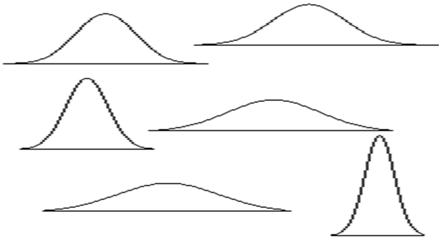
Characteristics of Normal Curves

• Most scores fall near the center, fewer at the extremes.
• Symmetrical.
  • Skewness = zero
• Mean, Median, Mode are all the same.
  • At the center.
• Dispersion can change.

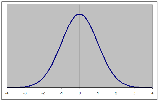
Standard Normal Curve

The Standard Normal Curve is a special case of the family of normal curves.

• Theoretical distribution (rather than Empirical distribution).
  • Meaning, it exists in theory and we assume it represents actual variables.
• Precisely defined by:
• So, the shape of the Standard Normal Curve is always the same (i.e., standardized).

Standard Normal Curve

• Does not exactly correspond to any distribution in nature.
  • However, most distributions in nature are assumed to closely resemble a normal curve.
• The scale (x-axis) has no limit above or below the mean (Re: Theoretical Distribution).
• It is always a `smooth' curve because as either a histogram or frequency polygon, the `intervals' of the scale are infinitesimal.

Why is it so common?

• Each raw score is influenced by many things, each of which is essentially random.
• The combination of these random influences is likely to be a middle score in most cases.
  • At or near the mean; unimodal.
• When not a middle score, there are equal chances of an imbalance of the random influences being in either direction (+ or -).
  • Symmetry; each extreme score in magnitude is as likely as one at the opposite end of the distribution.

Importance of the normal curve concept.

• Many of the variables we deal with are commonly assumed to be normally distributed in nature.
• If we can assume a variable is distributed approximately normally, then the techniques we discuss here allow us to make inferences about the phenomena we are studying (i.e., going from our study's sample data to the naturally occurring phenomena in the population using `traditional' statistical procedures).
  • Assuming normality allows us to assign probabilities.

Suspicion of Normality

• Central Limit Theorem (more on this later).
  • Mathematical Proof that an infinite number of random samples will create a normal distribution.
• Most traditional inferential statistical techniques have an assumption of normality which must be met in order to have confidence in the conclusions we come to, based on our sample results.
  • We must always consider this assumption.
  • Often we can test this assumption with objective criteria.
  • If we find the assumption violated, there are often modern (robust) analysis alternatives.

Central Limit Theorem

• If we draw an infinite number of repeated random samples (each with replacement), then we will end up with a normal distribution of sample means.
• The mean of that distribution (of means) will be the mean of the population.

http://onlinestatbook.com/simulations/CLT/clt.html

Why some distributions are not near normal.

• Limitations on minimum or maximum score possible.
  • Ceiling Effects such as percentage correct (max. = 100).
  • Floor Effects such as SAT scores of college students (only those with decent to high scores are in college).
• Limited number of categories.
  • Non-continuous variable; number of children in a family.
• Growth or time effects: children's height...age.
  • Some things are in constant growth or recession.
• Direct random effects: roulette wheel.
  • This has to do with probability, more on this later.

Normal Curve & Z-scores

• Because the normal curve is exactly defined...
• If a distribution is normal then there is an exact relation between any of its Z-scores and the percent of cases/scores above and below it.
  • If you know a particular Z-score, you can determine (often with a table) the percentage of scores above or below it.
  • If you know the percentages above and below, you can determine the Z-score.

Perfectly Symmetrical

• When dealing with the standard normal curve:
  • If a person has a Z-score of 0 (right at the mean), then we know 50% of the scores are above and 50% of the scores are below that point.
  • If a person has 50% of the scores above and 50% of the scores below, then we know that they have a Z-score of 0.
• The score itself has no area, it is simply a boundary between, a marker if you prefer.
  • Like in geometry, point and line are identifiers.

Z-scores along the bottom, the percentage of scores between each can be figured mathematically but, we use tables instead:
http://www.mathsisfun.com/data/standard-normal-distribution-table.html

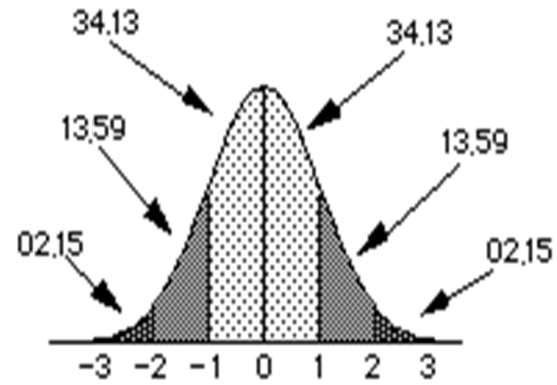
Z-scores along the bottom, percentages around the top
Memorize this image...burn it into your brain!!