|
XII.
Path
Analysis with Manifest Variables
First, let's take a moment to discuss and describe
our fictional* model. Our model consists of seven
directly measured variables or manifest variables. They include;
Education, Responsibility, Ambition, Wealth, Suggestibility, (Ethical)
Flexibility, and Political Success. Our model reflects hypothesized
causal relationships among characteristics of American politicians. Our
model hypothesizes three key causal variables (Wealth, Suggestibility,
& [Ethical] Flexibility) for political success. We further
expect politicians who exhibit high levels of education,
responsibility, and ambition to also exhibit greater wealth.
*Again; this is a fictional example and
is not meant to be taken seriously as a research finding supported by
empirical evidence. It is merely used here for instructional
example purposes.
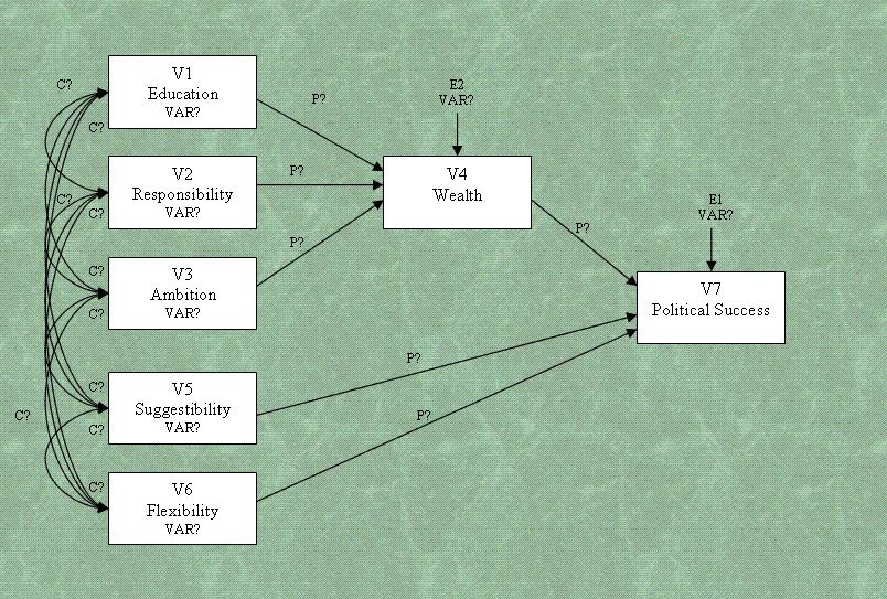
If you are unfamiliar with standard path and
structural equation models; there are a few things you should take note
of in our path diagram that tend to be seen in published materials
displaying path models and structural equation models. First, the use
of squares or rectangles to denote observed or measured variables
(often referred to as manifest variables). Second, the use of straight,
single headed arrows to denote hypothesized causal relationships (often
referred to as a paths). And third, the use of curved, double-headed
arrows to refer to bi-directional relationships (often referred to as
correlations or covariances). Specific hypotheses should be used to
clarify what the researcher expects to find (e.g. a very strong
positive relationship between Wealth & Education).
One of the key issues with Path Analysis and SEM
is the issue of overidentification. A model is said to be
overidentified if it contains more unique inputs (sometimes called
informations) than the number of parameters being estimated. In our
example, we have seven measured variables. We can apply the following
formula to calculate the number of unique inputs:
(1)
number of unique inputs = (p ( p + 1 ) ) / 2
where p = the number of manifest or measured
variables. Given this formula and our 7 manifest variables; we
calculate 28 unique inputs or informations which is greater than the
number of parameters we are estimating. Looking at the diagram, we see
10 covariances (C?), 6 paths (P?), 5 variable variances, and 2 error
variances (VAR?). Adding these up, we get 23 parameters to be
estimated. Remember too that path analysis and SEM require large sample
sizes. Several general rules have been put forth as lowest reasonable
sample size estimates; at least 200 cases at a minimum, at least 5
cases per manifest or measured variable, at least 400 cases, at least
25 cases per measured variable...etc. The bottom line is this; path
analysis and SEM are powerful when done with adequate large samples
-- the larger the better.
The procedure for conducting path analysis and/or
SEM in SAS is PROC CALIS; however, PROC CALIS needs to have the data
fed to it. There are three ways to 'feed' PROC CALIS the data, (1) a
correlation matrix with the number of observations and standard
deviations for each variable, (2) a covariance matrix, and (3) use of
the raw data as input. Here we will use the correlation matrix with
number of observations and standard deviations. You can import the raw
data to SAS using the Import Wizard to import the
Example
Data 5c file using the SPSS File (*.sav) source
option and the member name ex5c. Once imported, you can get the
descriptive statistics and correlations which you will need to run the
path analysis.
PROC CORR DATA=ex5c;
RUN;
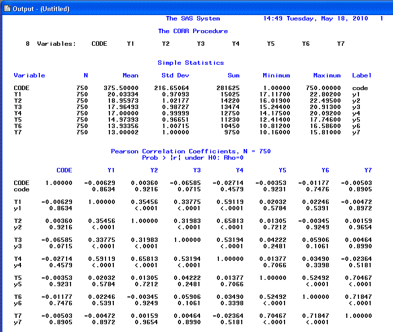
Using the number of observations (n =
750), the standard deviations, and the correlation matrix, you can
proceed to the path analysis.
The syntax for estimating or fitting our Path Model is displayed below.
Note that the top half of the syntax simply enters the data for the
path analysis. The bottom half (PROC CALIS) is used to fit the path
model.
DATA path1(TYPE=CORR);
INPUT _TYPE_ $ _NAME_ $ V1-V7;
LABEL
V1 = 'education'
V2 = 'responsibility'
V3 = 'ambition'
V4 = 'wealth'
V5 = 'suggestibility'
V6 = 'moral flexibility'
V7 = 'political success';
CARDS;
N . 750 750 750 750 750 750 750
STD . 0.9709 1.0218 0.9873 0.9999 0.9666 1.0072 1.0001
CORR V1 1.0000 . . . . . .
CORR V2 .3546 1.0000 . . . . .
CORR V3 .3377 .3198 1.0000 . . . .
CORR V4 .5912 .6581 .5319 1.0000 . . .
CORR V5 .0203 .0131 .0422 .0138 1.0000 . .
CORR V6 .0225 -.0034 .0591 .0349 .5249 1.0000 .
CORR V7 -.0047 .0016 .0046 -.0236 .7047 .7185 1.0000
;
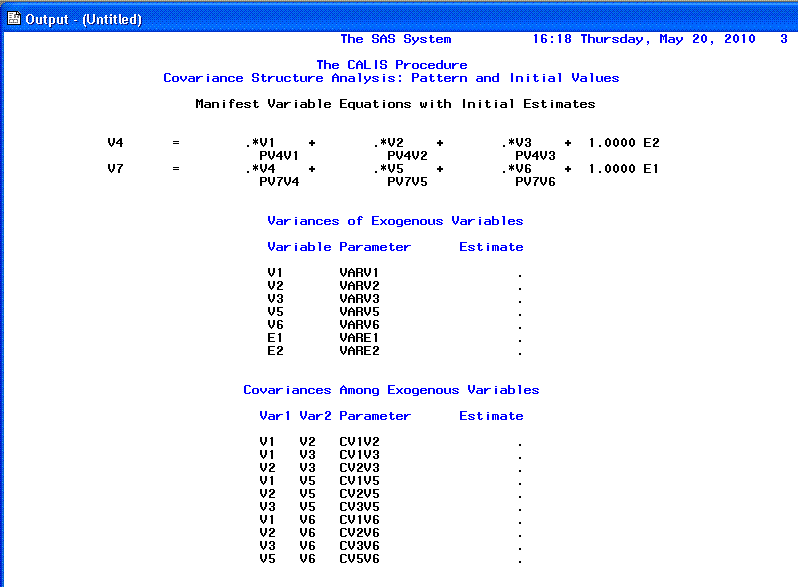
PROC CALIS COVARIANCE CORR RESIDUAL MODIFICATION ;
LINEQS
V7 = PV7V4 V4 + PV7V5 V5 + PV7V6 V6 + E1,
V4 = PV4V1 V1 + PV4V2 V2 + PV4V3 V3 + E2;
STD
E1 = VARE1,
E2 = VARE2,
V1 = VARV1,
V2 = VARV2,
V3 = VARV3,
V5 = VARV5,
V6 = VARV6;
COV
V1 V2 = CV1V2,
V1 V3 = CV1V3,
V1 V5 = CV1V5,
V1 V6 = CV1V6,
V2 V3 = CV2V3,
V2 V5 = CV2V5,
V2 V6 = CV2V6,
V3 V5 = CV3V5,
V3 V6 = CV3V6,
V5 V6 = CV5V6;
VAR V1 V2 V3 V4 V5 V6 V7;
RUN;
The PROC CALIS statement is followed by options.
First, COVARIANCE tells SAS we want to use the covariance matrix to
perform the analysis. Even though we are using the correlation matrix
as our data input, SAS calculates the covariance matrix for the PROC
CALIS. The CORR option specifies that we want the output to include the
correlation matrix or covariance matrix on which the analysis is run.
The RESIDUAL option allows us to see the absolute and standardized
residuals in the output. The MODIFICATION option tells SAS to print the
modification indices (e.g. Lagrange Multiplier Test). The next part of
the syntax, LINEQS, provides SAS with the specific linear equations
which specify the paths we want estimated. The first of which can be
read as: variables 7 is causally effected by the path between variable
7 and variable 4, the path between variable 7 and variable 5, the path
between variable 7 and variable 6, and the error variance associated
with variable 7. Next, we see the STD lines which specify which
variances we want estimated (listed as VAR here and in the diagram
above). Last, the COV statements specify all the covariances which need
to be estimated. Then, the VAR line simply lists the variables to be
used in the analysis.
*Please note; the first page of output was
produced by the PROC CORR directly after importing the data (above).
Therefore, the references to page numbers of output associated with the
PROC CALIS will begin on the second page (p. 2) of the total output
file (e.g. page 1 of the PROC CALIS output actually has the number 2 in
the top right corner). The page number discrepancy is noted here
because all PROC CALIS procedures tend to produce several pages of
output.
The first page of the PROC CALIS output consists
of general information, including the number of endogenous variables
(any variable with a straight single-headed arrow
pointing at it) and the number of exogenous variables (any variable without
any straight single-headed arrows pointing to it).
The second page of the PROC CALIS output consists
of a listing of the parameters to be estimated; essentially a review of
the specified model from the CALIS syntax.
The third page shows the general components of the
model (e.g. number of variables, number of informations, number of
parameters, etc.); as well as the descriptive statistics and covariance
matrix for the variables entered in the model.

The fourth page provides the initial parameter
estimates.

The fifth page includes the iteration history.
Often it is important to focus on the last line of the Optimization
results (left side of the middle of the page) which states whether or
not convergence criterion was satisfied. Also of importance is the
beginning of the predicted covariance matrix, which is used for
comparison to the matrix of association (original covariance matrix) to
produce residual values.
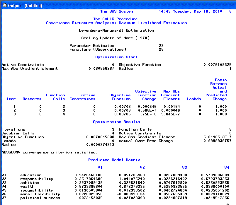
The sixth page continues the predicted covariance
matrix.

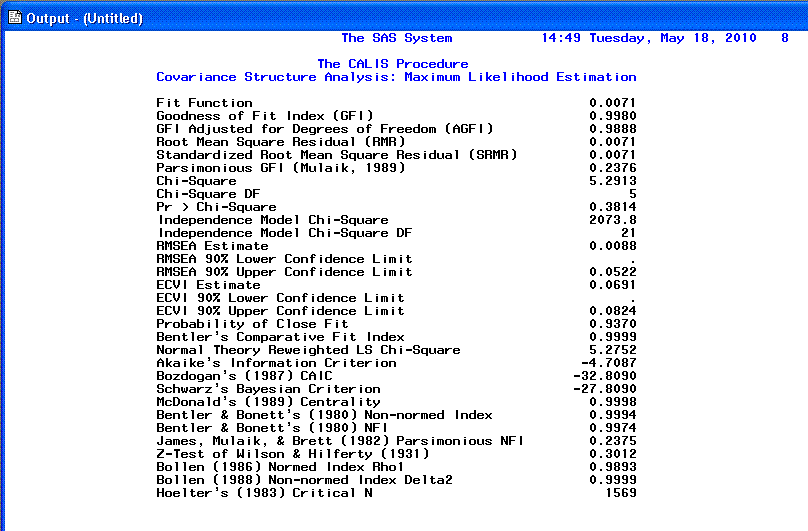
The seventh page displays fit indices. As you can
see, a fairly comprehensive list is provided. Please note that although
Chi-square is displayed it should not be used as an interpretation of
goodness-of-fit due to the large sample sizes necessary for path
analysis and SEM (which inflates the chi-square statistic to the point
of meaninglessness). Some of the more commonly reported fit indices are
the RMSEA (root mean square error of approximation), which when below
.05 indicates good fit; the Schwarz's Bayesian Criterion (also called
BIC; Bayesian Information Criteria), where the smaller the value (i.e.
below zero) the better the fit; and the Bentler & Bonnett's
Non-normed Index (NNFI) as well as the Bentler & Bonnett's
normed fit index (NFI)--both of which should be greater than .90 and
above to indicate good fit.
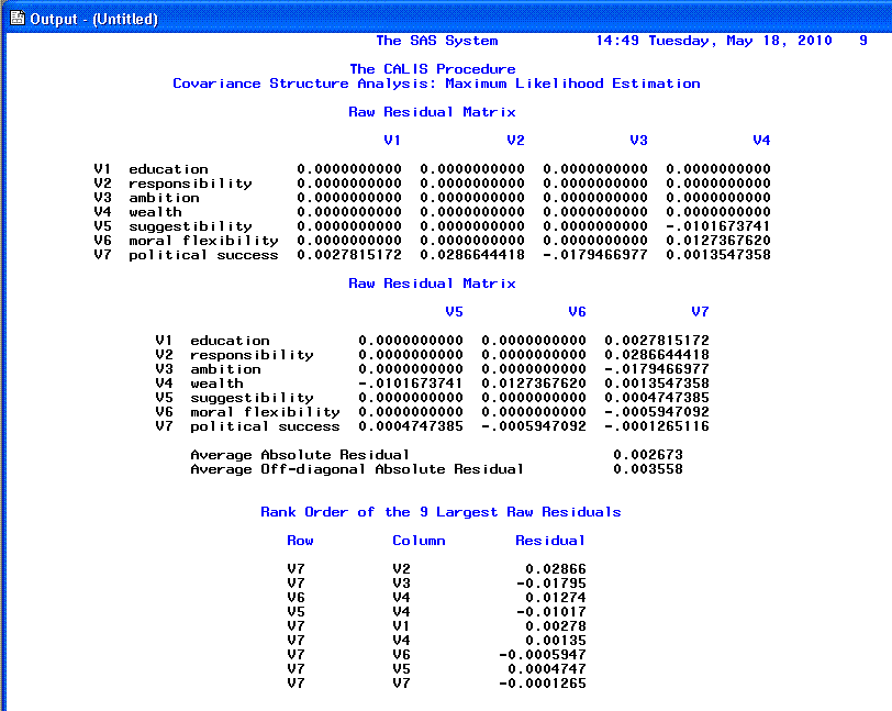
Page 8 provides the Raw
residual matrix and the ranking of the 9 largest
Raw residuals.
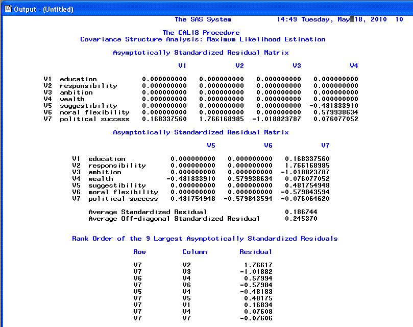
The 9th page shows the Standardized
residual matrix and the 9 largest
Standardized residuals; we expect values close to zero which
indicates good fit. Any values greater than |2.00| indicates lack of
fit and should be investigated.
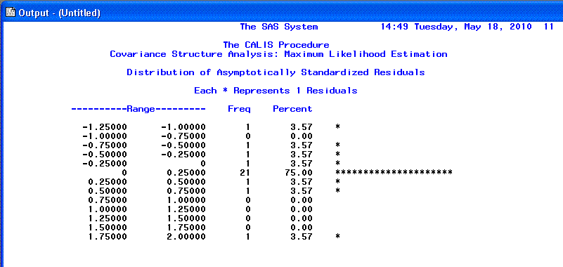
The 10th page displays a sideways histogram of the
distribution of the
Standardized residuals. Generally we expect to see a normal
distribution of residuals with no values greater than |2.00|.
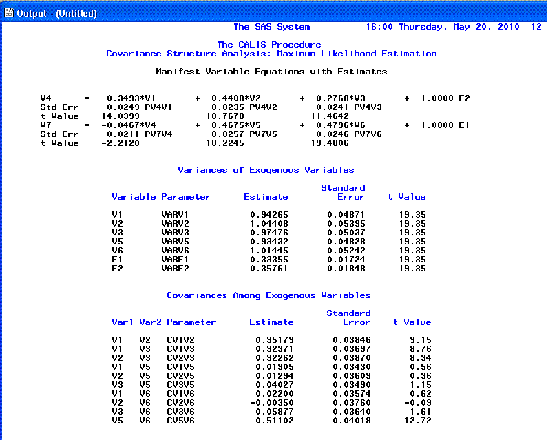
The 11th page displays our path coefficients in
Raw form, as well as t-values and standard errors
for the t-values associated with each. Further down
on the 11th page, we see estimated variance parameters and estimated
covariances; each with t-values and standard errors
for the t-values. Remember that t-values
for coefficients are statistically significant (p
< .05, two-tailed) if their absolute value is greater than 1.96;
meaning they are significantly different from zero. It is also
recommended that a review of the standard errors be performed, as
extremely small standard errors (those very close to zero) may indicate
a problem with fit associated with one variable being linearly
dependent upon one or more other variables.
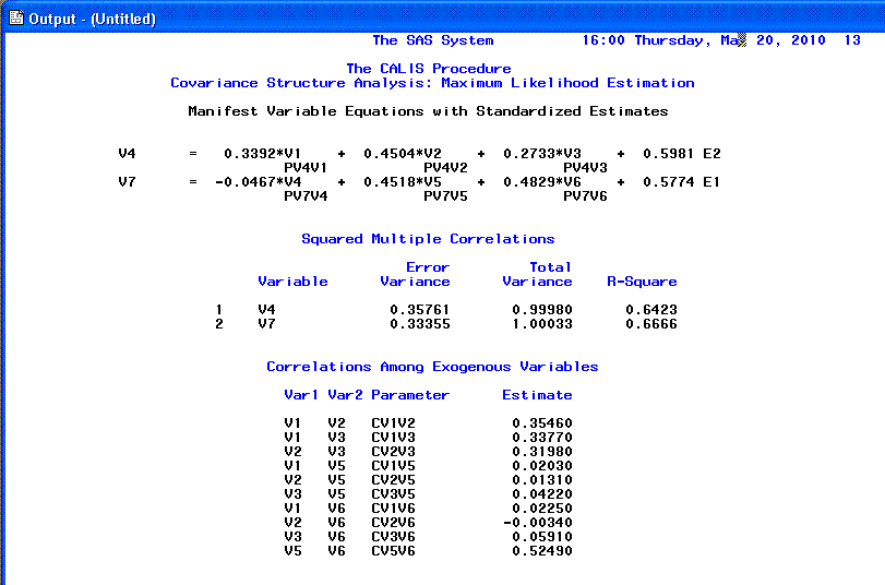
The 12th page provides Standardized path
coefficients and squared multiple correlations for endogenous variables
(often considered the dependent variables in such a model). The
'Squared Multiple Correlations' R-square column gives us an idea of how
well our model fits because, these values are interpreted as the
percentage of variance in our endogenous variables accounted for by
their respective exogenous variables. As an example; we could interpret
V7 (Political Success) as having 66.66% of its variance accounted for
by the combination of V4 (Wealth), V5 (Suggestibility), and V6 (Ethical
Flexibility).
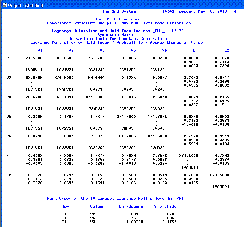
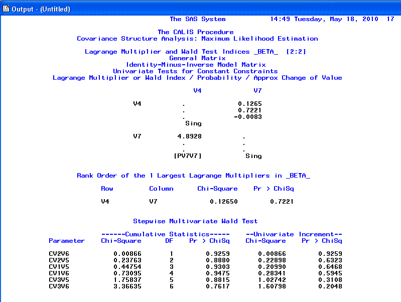
The 13th page begins the listing of the
modification indices, which continues to the end of the output. One
should be careful when interpreting modification indices and should do
so only after carefully interpreting all the previous output first.
Modification indices generally take two forms; ones which recommend the
exclusion of a parameter from the specified model and ones which
recommend inclusion of a parameter to the model. Both types attempt to
estimate the decrease in chi-square associated with the recommendation
being implemented (i.e. increased goodness of fit). However, as
mentioned above, chi-square is generally not an acceptable measure of
goodness-of-fit and therefore modification indices should be treated
with caution.
The 14th page.
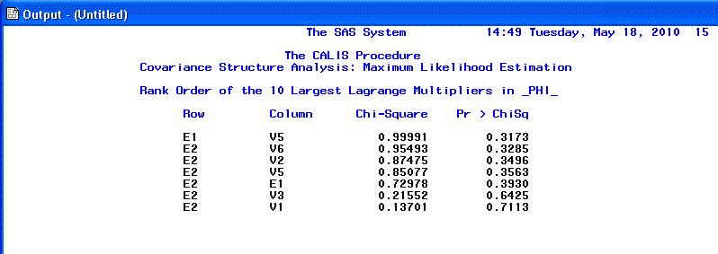
The 15th page.

The 16th page.
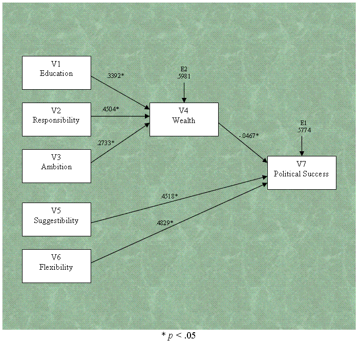
Below you will find our completed path diagram
with standardized path coefficients.
Generally speaking, the output for any PROC CALIS
will follow the same format seen here for path analysis; for example,
the order of the output's presentation will be the same for the SEM
example in the next tutorial.
Please realize this tutorial is
not meant to be an exhaustive review; it is merely an introduction.
This tutorial is not meant to replace one or several good textbooks.
And that concludes the tutorial on Path Analysis with manifest
variables.
The tutorial on the basics of Structural Equation
Modeling (SEM) can be found
here.
|