|
If you are not familiar with SEM it is strongly recommended you work
your way through the
Path
Analysis tutorial and example prior to working through this
tutorial and example.
XIII. Structural
Equation Modeling
(SEM) using PROC CALIS
First, let's take a moment to discuss and describe
our fictional* model. Our model consists of 13
manifest variables which are assumed to measure four latent factors.
The first latent factor, Personality, is assumed to be measured by
Extroversion (extro), Openness (open), and Agreeableness (agree). The
second latent factor, Engagement, is assumed to be measured by Social
Engagement (social), Cognitive Engagement (cognitive), Physical
Engagement (physical), and Cultural Engagement (cultural). The third
latent factor, Crystallized Intelligence, is assumed to be measured by
the established tests of Vocabulary (vocab), Abstruse Analogies
(abstruse), and Block Design (block). The fourth latent factor, Fluid
Intelligence, is assumed to be measured by the established tests of
Common Analogies (common), Letter Sets (sets), and Letter Series
(series). The general research question for our fictional longitudinal
study concerns whether or not certain personality traits cause persons
to lead an engaged lifestyle, and do these personality traits and
leading an engaged lifestyle prevent loss of cognitive functioning in
late life (e.g. beyond 65 years of age).
*Again; this is a fictional example; it
includes simulated data and is not meant to be taken seriously as a
research finding supported by empirical evidence. It is
merely used here for instructional example purposes.
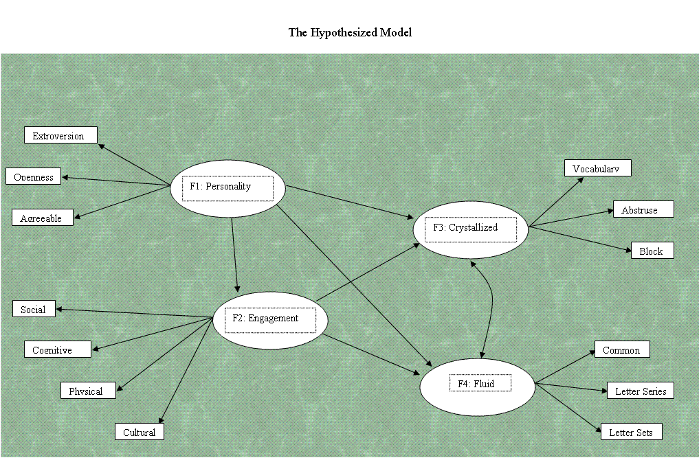
If you are unfamiliar with standard path and
structural equation models; there are a few things you should take note
of in our diagram that tend to be seen in published materials
displaying path models and structural equation models. First, the use
of squares or rectangles to denote observed or measured variables
(often referred to as manifest variables or indicator variables).
Second, the use of circles or ellipses to denote unobserved or latent
variables (often referred to as latent factors). Third, the use of
straight, single headed arrows to denote causal relationships. There
are two types of causal relationships shown in most diagrams. The
assumed causal relationship between a latent factor and its indicator
or manifest variables which are often referred to as loadings or factor
loadings or factor coefficients. The hypothesized causal relationship
between two latent factors which are often referred to as paths or path
loadings or path coefficients. And fourth, the use of curved,
double-headed arrows to refer to bi-directional relationships (often
referred to as correlations or covariances). Specific hypotheses should
be used to clarify what the researcher expects to find (e.g. a positive
bi-directional relationship or correlation between Crystallized
& Fluid Intelligences).
Please note: From this point
forward, we will use the term loading to refer to a
relationship between a manifest variable and a latent factor. We will
use the term path to refer to the relationship
between two latent factors.
Something to consider when conducting SEM is the
recommendation of using a two stage process to conduct the SEM
(Anderson & Gerbing, 1988). When using two stages, the first
stage is used to verify the measurement model. Verification of the
measurement model in SEM can be considered analogous to conducting a
confirmatory factor analysis. The purpose is to ensure you are
measuring (adequately) what you believe you are measuring. Essentially,
you are verifying the factor structure. When verifying the measurement
model, you are more concerned with the error variances and the loadings
than with the relationships between latent factors
(paths). Recall, the loadings are those which represent the
relationships between a factor and its manifest indicator variables.
The second stage involves actually testing the hypothesized causal
relationships between factors, also referred to as testing the
structural model, which is where you are interested more in the paths
than the loadings. Recall, the paths represent the hypothesized causal
relationships between latent factors.
# Anderson, J. C., & Gerbing, D. W.
(1988). Structural equation modeling in
# practice: A review
and recommended two-step approach. Psychological
# Bulletin,
103, 411 - 423.
Stage I: Verifying the Measurement model.
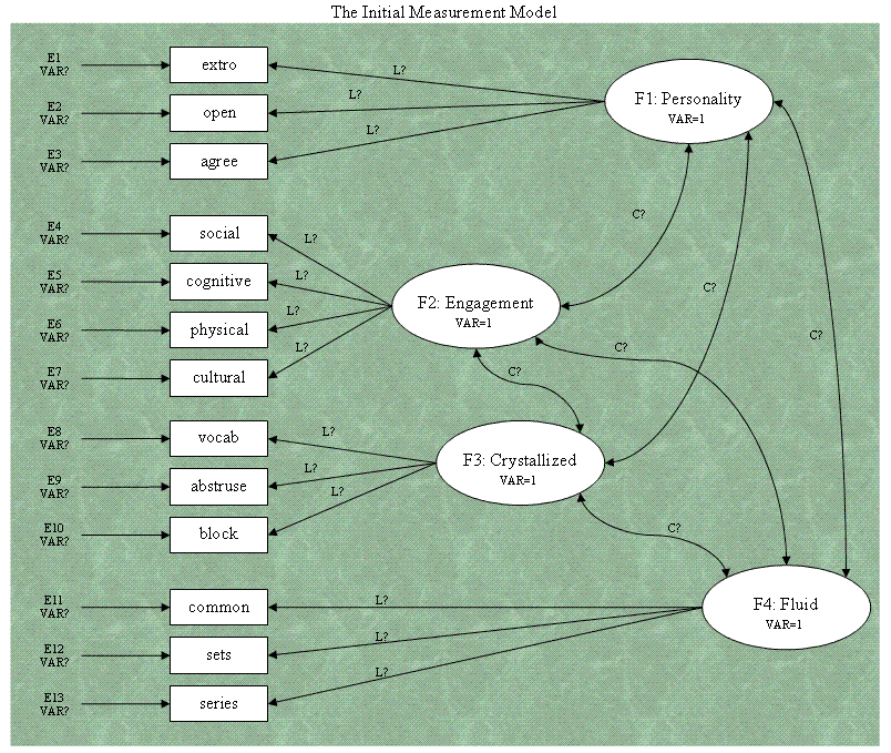
Below you'll find a diagram which represents our
measurement model. Notice we are unconcerned with the relationships
between latent factors, those paths are free to vary (estimating the
correlations or covariances) without specifying hypothetical causal
relationships between them. Also notice, the variances of the factors
are fixed at 1. Remember, the latent factors are unobserved and
therefore we do not have an idea of their variance, nor their scale.
Another thing to notice is that each observed score (i.e. manifest
variable) is caused by a latent factor which we believe we are
measuring indirectly, and measurement error. These
error terms are shown in the diagram with arrows pointing toward the
manifest variables as classical test theory suggests (i.e. observed
score = true score + measurement error). This bears mentioning because
it is one of the reasons SEM is so popular; it allows us to model
measurement error.
One of the key requirements of Path Analysis and
SEM is overidentification. A model is said to be overidentified if it
contains more unique inputs (sometimes called informations) than the
number of parameters being estimated. In our example, we have 13
manifest variables. We can apply the following formula to calculate the
number of unique inputs:
(1)
number of unique inputs = (p ( p + 1 ) ) / 2
where p = the number of manifest variables. Given
this formula and our 13 manifest variables; we calculate 91 unique
inputs or informations which is greater than the number of parameters
we are estimating. Looking at the diagram, we see 6 covariances (C?),
13 loadings (L?), and 13 error variances (VAR?). Adding these up, we
get 32 parameters to be estimated. You'll notice that for our
measurement model, we have specified the variance of the latent factors
to be 1 (VAR=1). This is done to allow estimation of all the factor
loadings. Remember too that path analysis and SEM require large sample
sizes. Several general rules have been put forth as lowest reasonable
sample size estimates; at least 200 cases at a minimum, at least 5
cases per manifest or measured variable, at least 400 cases, at least
25 cases per measured variable, 5 observations or cases per parameter
to be estimated, 10 observations or cases per parameter to be
estimated...etc. The bottom line is this; path analysis and SEM are
powerful when done with adequately large samples -- the
larger the better. Another issue related to sample size, is the
recommendation of having at least 3 manifest variables for each latent
factor; with the suggestion of having 4 or more manifest variables for
each latent factor (Anderson & Gerbing, 1988). Having 4 allows
you the flexibility to delete one if you find it does not contribute
meaningfully to a latent factor or the model in general (e.g. it loads
on more than one factor to a meaningful extent). Another consideration
is that of remaining realistic when setting out to study a particular
phenomena with SEM in mind as the analysis. It is often easy to develop
some very complex models containing a great number of manifest
variables. However, complex models containing more than 20 manifest
variables can lead to confusion in interpretation and a lack of fit, as
well as convergence difficulty. Bentler and Chou (1987) recommend a
limit of 20 manifest variables.
# Bentler, P. M., & Chou, C. (1987).
Practical issues in structural modeling.
Sociological
# Methods
& Research, 16, 78 - 117.
The procedure for conducting SEM in SAS is PROC
CALIS; however, PROC CALIS needs to have the data fed to it. There are
three ways to 'feed' PROC CALIS the data, (1) a correlation matrix with
the number of observations and standard deviations for each variable,
(2) a covariance matrix, and (3) use of the raw data as input. Here we
will use the correlation matrix with number of observations and
standard deviations. Use the Import Wizard to import the
SEM
Data file using the SPSS File (*.sav) source option
and member name semd.
Once imported, you can get the descriptive
statistics and correlations which you will need to run the SEM
analysis.
PROC CORR DATA=semd;
RUN;
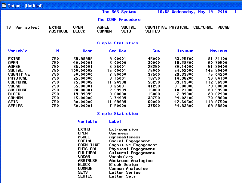
Note, there are 3 pages of output for the PROC
CORR. The first page shows the descriptive statistics, variable names,
and variable labels.
The second and third pages show the correlation
matrix.
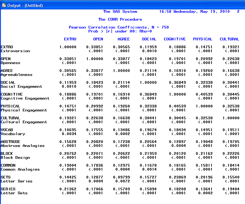
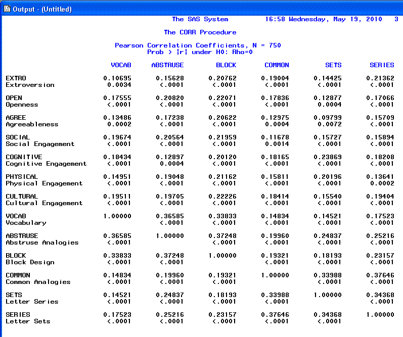
Using the number of observations (n =
750), the standard deviations, and the correlation matrix, you can
proceed to the SEM.
The syntax for estimating or fitting our Measurement Model is displayed
below. Note that the top half of the syntax simply enters the data; the
second half (beginning with PROC CALIS) is used to conduct the SEM.
DATA sem1(TYPE=CORR);
INPUT _TYPE_ $ _NAME_ $ V1-V13;
LABEL
V1 = 'extro'
V2 = 'open'
V3 = 'agree'
V4 = 'social'
V5 = 'cognitive'
V6 = 'physical'
V7 = 'cultural'
V8 = 'vocab'
V9 = 'abstruse'
V10 = 'block'
V11 = 'common'
V12 = 'sets'
V13 = 'series'
;
CARDS;
N . 750 750 750 750 750 750 750 750 750 750 750 750 750
STD . 9.0000 6.0000 5.2500 15.0000 7.5000 3.7500 11.2500 8.2500 3.0000
3.0000 6.7500 12.0000 7.5000
CORR V1 1.0000 . . . . . . . . . . . .
CORR V2 .3385 1.0000 . . . . . . . . . . .
CORR V3 .3056 .3388 1.0000 . . . . . . . . . .
CORR V4 .1196 .1842 .2111 1.0000 . . . . . . . . .
CORR V5 .1889 .1970 .1691 .3685 1.0000 . . . . . . . .
CORR V6 .1475 .2099 .1926 .3234 .4054 1.0000 . . . . . . .
CORR V7 .1932 .2264 .1664 .3044 .3044 .3254 1.0000 . . . . . .
CORR V8 .1070 .1755 .1349 .1967 .1843 .1495 .1951 1.0000 . . . . .
CORR V9 .1563 .2082 .1724 .2056 .1290 .1905 .1971 .3659 1.0000 . . . .
CORR V10 .2076 .2207 .2062 .2196 .2012 .2116 .2223 .3383 .3725 1.0000 .
. .
CORR V11 .1900 .1784 .1298 .1168 .1816 .1581 .1841 .1483 .1996 .1932
1.0000 . .
CORR V12 .1443 .1288 .0980 .1573 .2387 .2020 .1554 .1452 .2484 .1819
.3399 1.0000 .
CORR V13 .2136 .1707 .1571 .1589 .1821 .1364 .1940 .1752 .2522 .2316
.3765 .3437 1.0000
;
PROC CALIS COVARIANCE CORR RESIDUAL MODIFICATION;
LINEQS
V1 = LV1F1 F1 + E1,
V2 = LV2F1 F1 + E2,
V3 = LV3F1 F1 + E3,
V4 = LV4F2 F2 + E4,
V5 = LV5F2 F2 + E5,
V6 = LV6F2 F2 + E6,
V7 = LV7F2 F2 + E7,
V8 = LV8F3 F3 + E8,
V9 = LV9F3 F3 + E9,
V10 = LV10F3 F3 + E10,
V11 = LV11F4 F4 + E11,
V12 = LV12F4 F4 + E12,
V13 = LV13F4 F4 + E13;
STD
F1 = 1,
F2 = 1,
F3 = 1,
F4 = 1,
E1-E13 = VARE1-VARE13;
COV
F1 F2 = CF1F2,
F1 F3 = CF1F3,
F1 F4 = CF1F4,
F2 F3 = CF2F3,
F2 F4 = CF2F4,
F3 F4 = CF3F4;
VAR V1-V13;
RUN;
The PROC CALIS statement is followed by options.
First, COVARIANCE tells SAS we want to use the covariance matrix to
perform the analysis. Even though we are using the correlation matrix
as our data input, SAS calculates the covariance matrix for the PROC
CALIS. That is why the number of observations and standard deviations
must be included with the correlations. The CORR option specifies that
we want the output to include the correlation matrix or covariance
matrix on which the analysis is run. The RESIDUAL option allows us to
see the absolute and standardized residuals in the output. The
MODIFICATION option tells SAS to print the modification indices (e.g.
Lagrange Multiplier Test). The next part of the syntax, LINEQS,
provides SAS with the specific linear equations which specify the
loadings we want estimated. The first of which can be read as: variable
1 equals factor 1 and the error variance associated with variable 1.
Next, we see the STD lines which specify which variances we want
estimated. Notice here we have fixed the variance of each factor at 1,
as discussed above. The error variances are being estimated as VARE1
through VARE13. Last, the COV statements specify all the covariances
which need to be estimated. Then, the VAR line simply lists the
variables to be used in the analysis; V1 through V13. Pay particular
attention to the location of commas and semi-colons.
*Please note; the first 3 pages
of output was produced by the PROC CORR directly after importing the
data (above). Therefore, the references to page numbers of output
associated with the PROC CALIS will begin on the fourth page (p. 4) of
the total output file (e.g. page 1 of the PROC CALIS output actually
has the number 4 in the top right corner). The page number discrepancy
is noted here because all PROC CALIS procedures tend to produce several
pages of output.
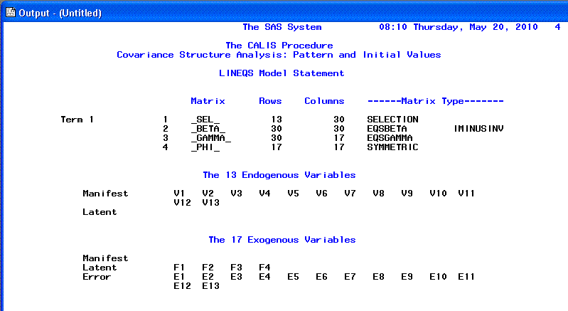
The first page of the PROC CALIS output consists
of general information, including the number of endogenous variables
(any variable with a straight single-headed arrow
pointing at it) and the number of exogenous variables (any variable without
any straight single-headed arrows pointing to it). An important point
to notice here is that the factors are listed as exogenous variables,
even though they have arrows pointing to them, those arrows are double
headed and indicate relationship without causation. Meaning, the
factors may be related, but are not caused by anything specified in our
model (more specifically by our line equations). This may help clarify
the use of the word exogenous -- which in SEM
terminology refers to variables which have causes outside
the model.
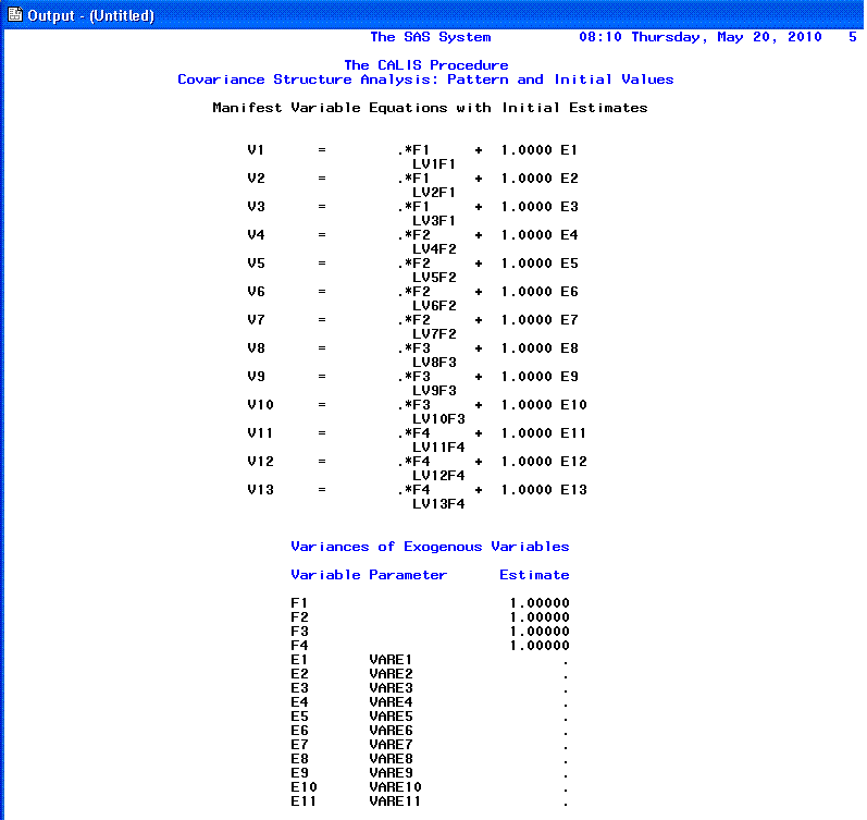
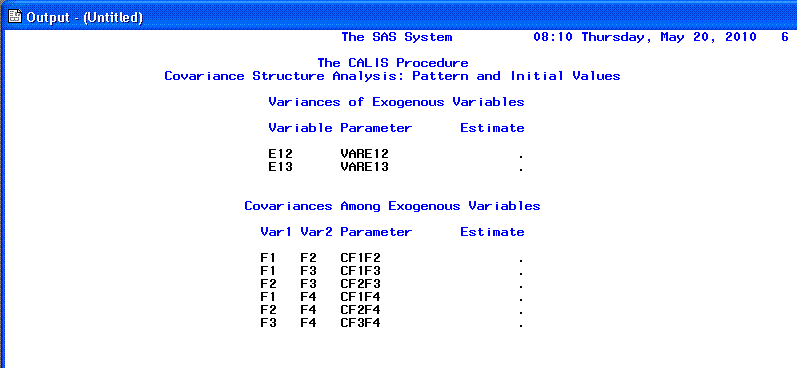
The second and third pages of the PROC CALIS
output consist of a listing of the parameters to be estimated;
essentially a review of the specified model from the CALIS syntax.
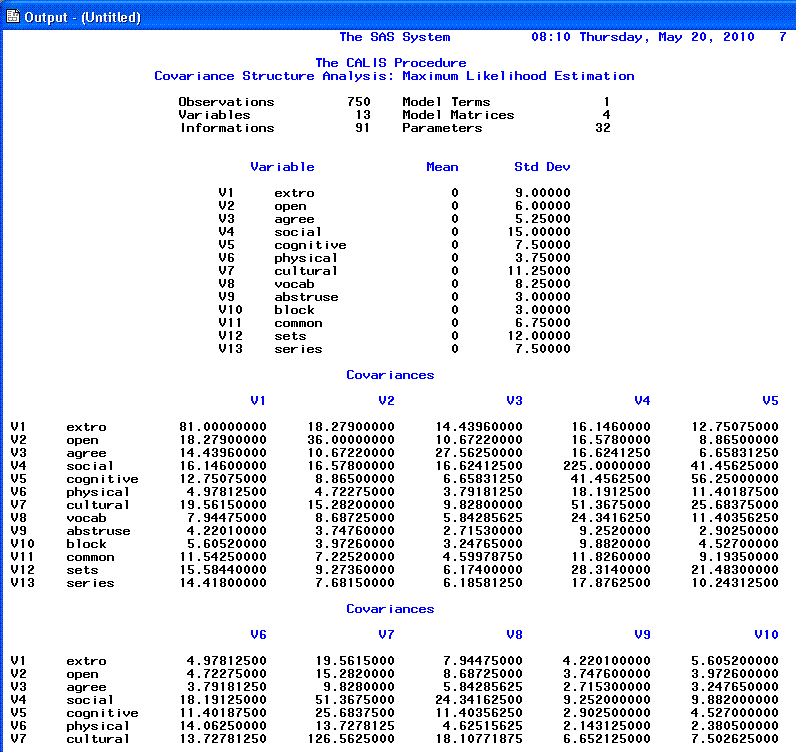
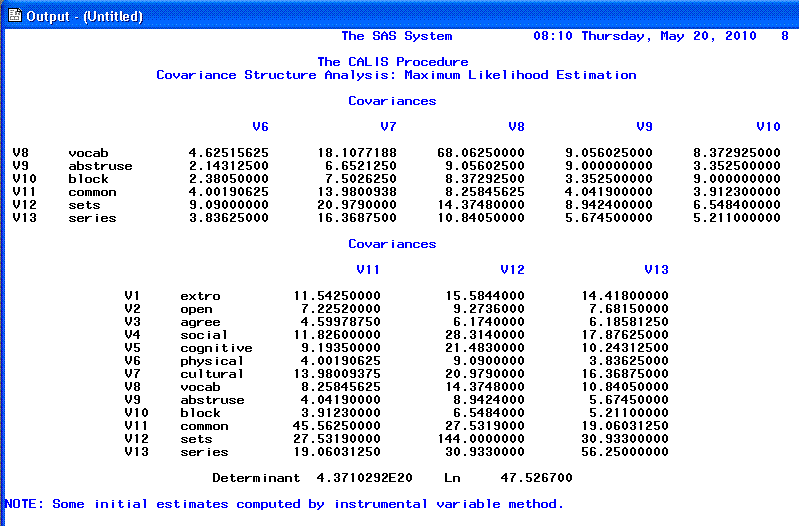
The fourth and fifth pages show the general
components of the model (e.g. number of variables, number of
informations, number of parameters, etc.); as well as the descriptive
statistics and covariance matrix for the variables entered in the
model. The covariance matrix starts on the fourth page (p. 7) and
continues onto the fifth page (p. 8).
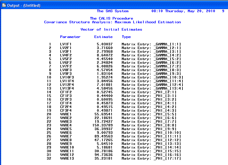
The 6th page provides the initial parameter
estimates.
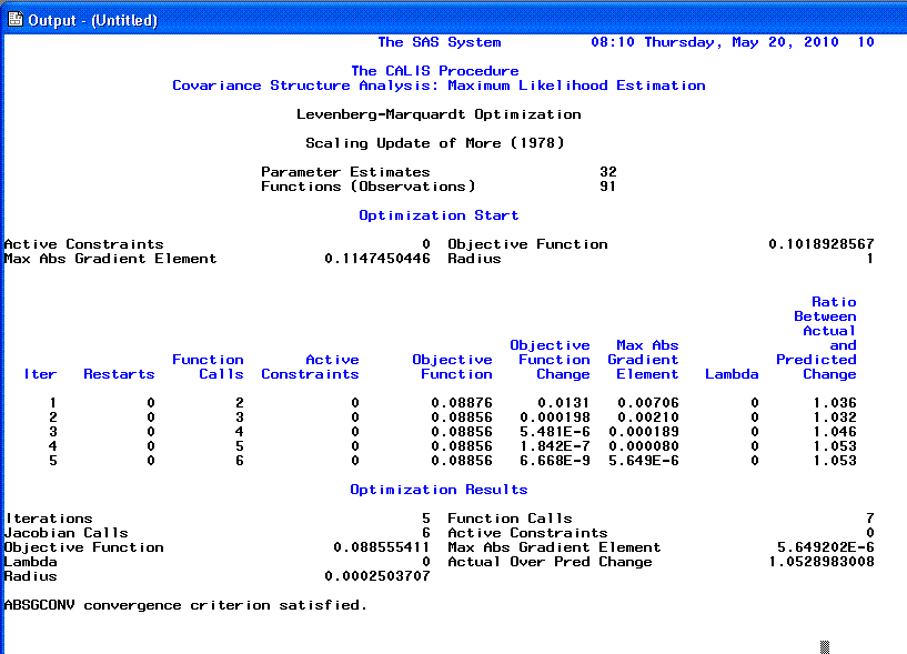
The 7th page includes the iteration history. Often
it is important to focus on the last line of the Optimization results
(left side of the bottom of the page) which states whether or not
convergence criterion was satisfied.
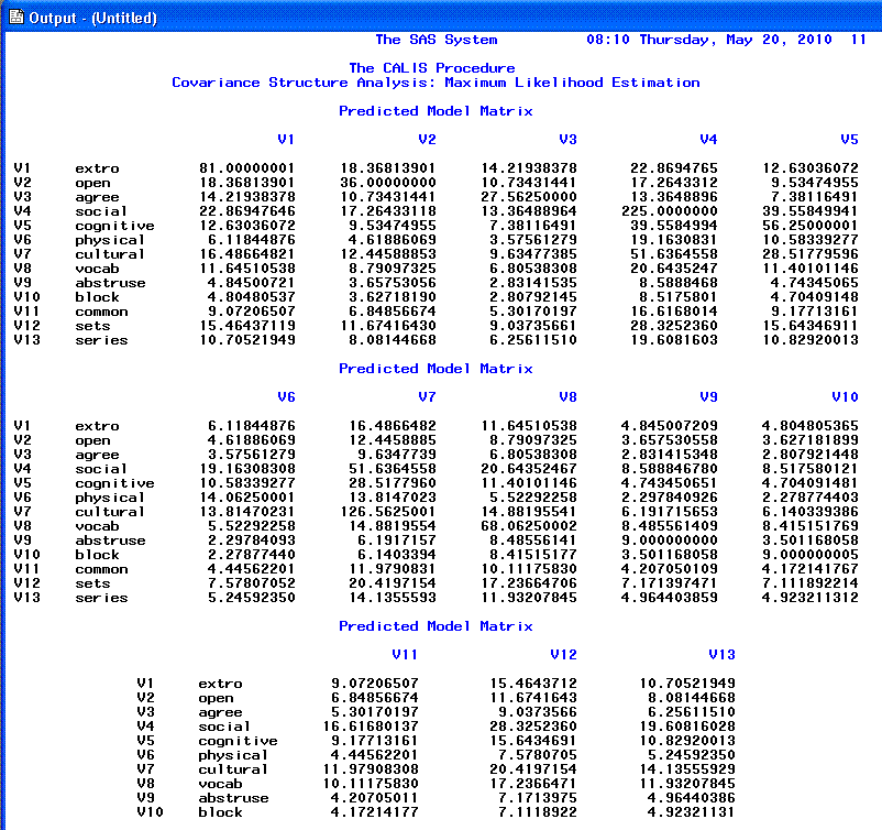
The 8th and 9th pages contain the predicted
covariance matrix, which is used for comparison to the matrix of
association (original covariance matrix) to produce residual values.

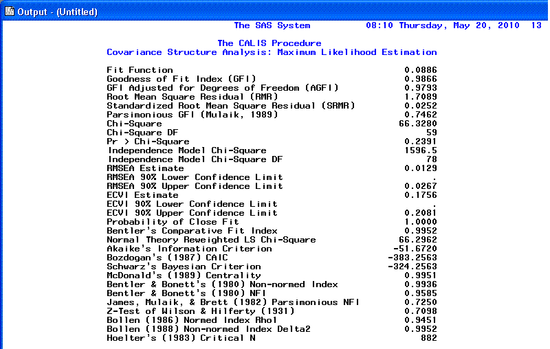
The 10th page displays fit indices. As you can
see, a fairly comprehensive list is provided. Please note that although
Chi-square is displayed it should not be used as an interpretation of
goodness-of-fit due to the large sample sizes necessary for SEM (which
inflates the chi-square statistic to the point of meaninglessness).
Some of the more commonly reported fit indices are the RMSEA (root mean
square error of approximation), which when below .05 indicates good
fit; the Schwarz's Bayesian Criterion (also called BIC; Bayesian
Information Criteria), where the smaller the value (i.e. below zero)
the better the fit; and the Bentler & Bonnett's Non-normed
Index (NNFI) as well as the Bentler & Bonnett's normed fit
index (NFI)--both of which should be greater than .90 and above to
indicate good fit.
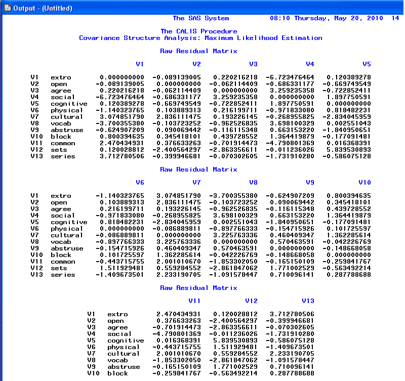
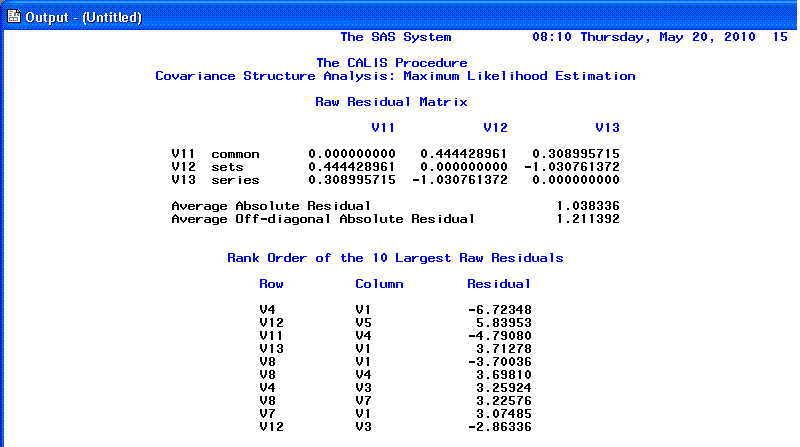
Page 11 and 12 provide the Raw
residual matrix and the ranking of the 10 largest
Raw residuals.
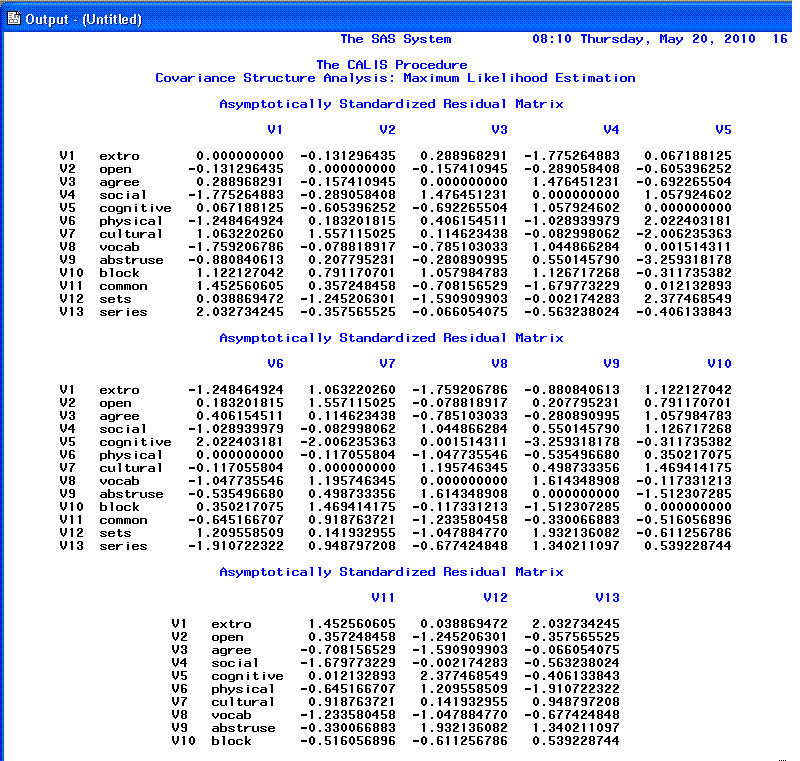
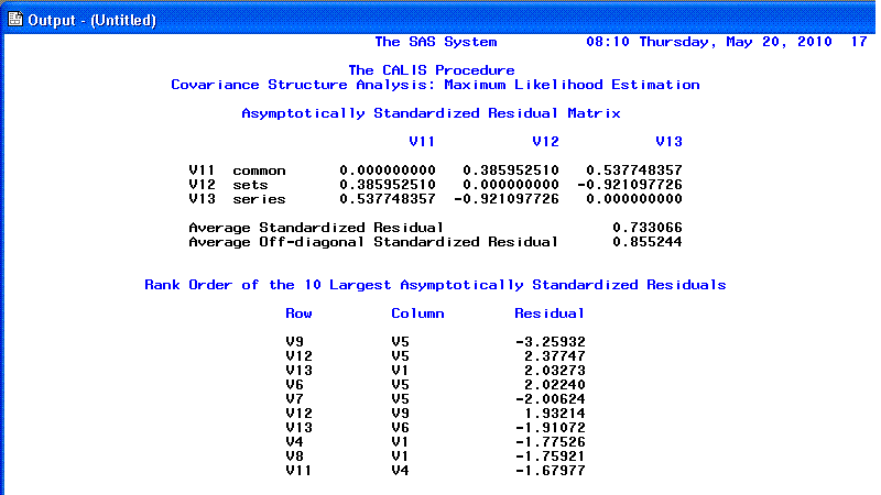
The 13th and 14th pages show the Standardized
residual matrix and the 10 largest
Standardized residuals; we expect values close to zero which
indicates good fit. Any values greater than |2.00| indicates lack of
fit and should be investigated. This is really the heart of evaluating
goodness of fit; if fit is truly good, you would see virtually no
difference between the original covariance matrix and the predicted
covariance matrix (i.e. each of the residuals would be zero).
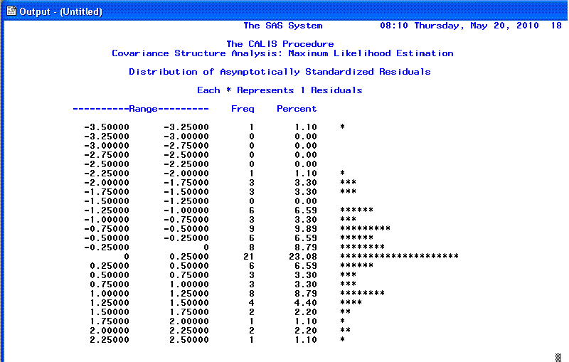
The 15th page displays a sideways histogram of the
distribution of the
Standardized residuals. Generally we expect to see a normal
distribution of residuals with no values greater than |2.00|.
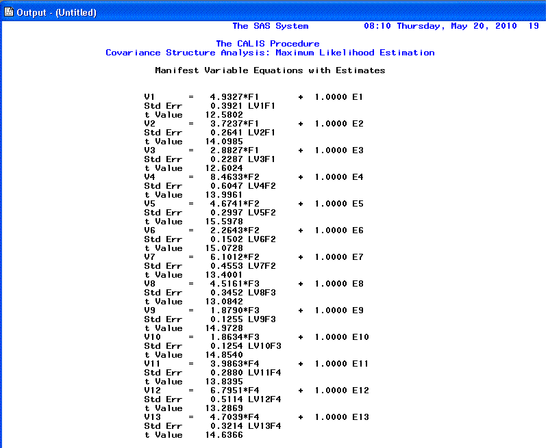
The 16th page displays our loadings (coefficients)
in Raw form, as well as t-values and standard
errors for the t-values associated with each.
Remember that t-values for coefficients (here
loadings) are statistically significant (p <
.05, two-tailed) if their absolute value is greater than 1.96; meaning
they are significantly different from zero. If the t-value
is greater than 2.58, then p < .01 and if
the t-value is greater than 3.29, then
p < .001. It is also recommended
that a review of the standard errors be performed, as extremely small
standard errors (those very close to zero) may indicate a problem with
fit associated with one variable being linearly dependent upon one or
more other variables. Here, all our t-values for
our factor loadings are greater than 3.29 and none of our standard
errors are noticeably low (i.e. less than .0099 for instance).
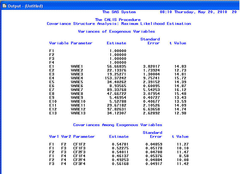
On the 17th page, we see estimated variance
parameters and estimated "Covariances" (which are really correlations);
each with t-values and standard errors for the t-values.
Notice at the top the variance estimates table, our factor variances
are fixed (from our syntax) at 1.0000.
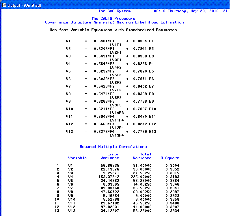
The 18th page provides Standardized
factor loadings (coefficients; analogous to
β)
and squared multiple correlations. The 'Squared Multiple Correlations'
R-square column gives us an idea of how well our manifest variables
reflect the latent factors because, these values are interpreted as the
percentage of variance accounted for in our manifest variables by their
respective factors. As an example; we could interpret V1 (Extroversion)
as having 30.004% of its variance accounted for by F1 (Personality).
You'll notice, the R?
value is simply the square of the loading (e.g. .5481? = .3004).
Furthermore, if we square our E1 term (.8364), we get .6996, which when
added to the variance accounted for by the factor (.3004) gives us the
complete standardized variance of our V1 variable: 1.00. This confirms
our classical test theory perspective of observed score = true score
(the amount of the latent factor) + error.
The 19th page again shows us the correlations
between our factors (as was displayed previously on the the bottom of
the 17th page).

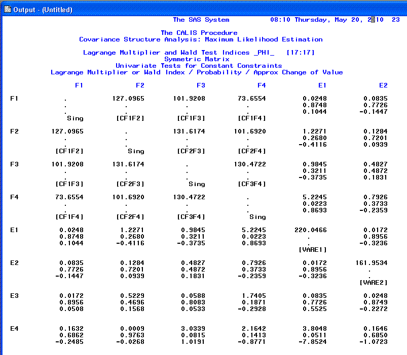
The 20th page begins the listing of the
modification indices, which continues to the end of the output. One
should be careful when interpreting modification indices and should do
so only after carefully interpreting all the previous output first.
Modification indices generally take two forms; ones which recommend the
exclusion of a parameter from the specified model (the Wald Test) and
ones which recommend inclusion of a parameter to the model (the
Lagrange Multiplier). Both types attempt to estimate the change in
chi-square associated with the recommendation being implemented (i.e.
increased goodness of fit). However, as mentioned above, chi-square is
generally not an acceptable measure of goodness-of-fit and therefore
modification indices should be treated with caution. For this reason,
the remaining pages of output (displaying modification indices) will
not be shown here.
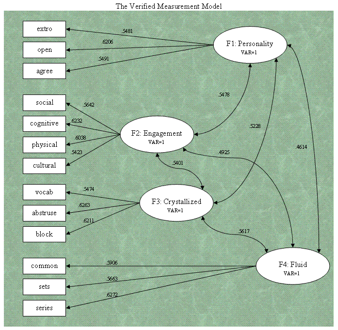
The completed diagram of the verified Measurement
Model is below. Note, typically standardized factor loadings are
reported (rather than un-standardized) and error terms are generally
not reported in diagrams -- as is the case below.
Generally speaking, the output for any PROC CALIS
will follow the same format seen here for SEM analysis; for example,
the order of the output's presentation will be the same for the example
in the next tutorial which shows the second stage of SEM;
testing
the structural model.
Please realize, this tutorial
is not an exhaustive review, merely an introduction. It is not meant to
be a replacement for one or several good textbooks.
|


