MODULE 6

Task: Conduct Multiple Imputation for missing values using a version of the Estimation Maximization (EM) algorithm. The user manual for the Missing Values module can be found at the SPSS Manuals page. For a more detailed treatment of the more general topic of missing value analysis, see Little and Rubin (1987).

The SPSS Missing Values module is implemented in two distinct ways. First, the Missing Values Analysis (MVA) menu option produces a series of tables and figures which describe the pattern of missingness, estimates of basic descriptive statistics (means, standard deviations, correlations, covariances) based on a user specified method (e.g. EM), and imputes values based on the specified method. It is important to note that this approach can be referred to as single or simple imputation; rather than multiple imputation, which is widely accepted as superior. To read about why this simple imputation is not a good idea, see Von Hippel (2004). The second (newer) way the module is implemented is through the use of the Multiple Imputation menu option which itself contains two menu options (i.e. functions): Analyze Patterns and Impute Missing Data Values. These two options will be covered below.

Start off by importing the DataMissing.sav file into the Data Editor window of SPSS. The data is simulated (i.e. fictitious) and was generated originally with all the values intact. Subsequently, a function was used to randomly remove approximately 5% of the values (using the statistical programming environment R). The data contains 18 variables; one case identification variable, five categorical variables (nominal and ordinal scaled), and twelve continuous or nearly continuous variables (considered interval or ratio scaled). The data contains 1500 cases. 

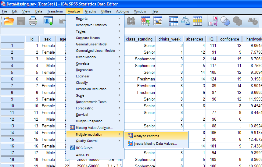
1.) Evaluation of Missing Values

First, click on "Analyze", then "Multiple Imputation", then "Analyze Patterns..." in the toolbar at the top of SPSS.

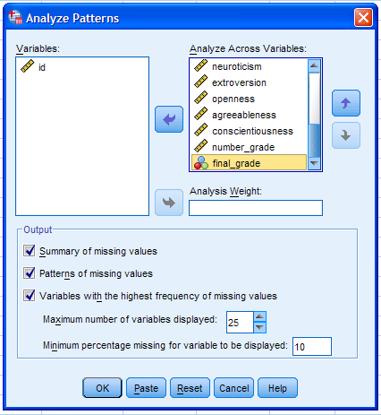
Next, select all the variables (excluding the case identification variable) and move them to the Analyze Across Variables: box. There are only 17 variables included in the analysis so the maximum number of variables displayed (25) will display all the variables included. Further control over what is displayed in the output can be exercised by changing the minimum percentage missing cutoff value. 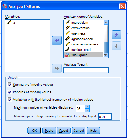The default (10%) indicates that only variables with 10% or more missing values will be displayed in the output. Since it is generally good practice to review all the patterns of missingness, we will change the percentage cutoff to 0.01% -- thus insuring all variables are included in the output (right figure below). Then, we can click the OK button to proceed.

The following output was produced.

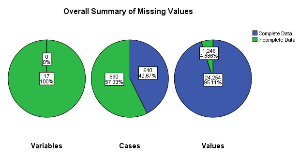
First, a figure with three pie charts displays the number and percentage of missing variables (left), cases (center), and individual cells (right) which have at least one missing value. Note that green indicates missing; for instance, the Variables (left) pie indicates that 17 variables (100% of those included in the analysis) have at least one missing value. The Cases (middle) pie indicates 860 (57.33%) of the 1500 cases contained at least one missing value. The Values (right) pie indicates that approximately 5% of all values are missing (i.e. 17 variables multiplied by 1500 cases equals 25500 values, so 1246 equals 4.886% missing).

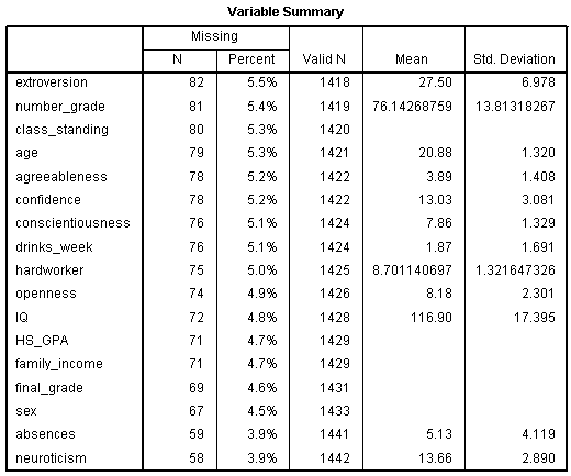
Next, the Variable Summary chart displays the (as specified) variables which contained at least 0.01% missing values. The number of missing values, percentage missing, number of valid values, mean based on valid values, and standard deviation based on valid values are displayed for each of the 17 variables. Notice, the variables are ordered by the amount of values they are missing (i.e. the percentage missing). Extroversion is listed first because it has the highest percentage of missing values (5.5%). Neuroticism is listed last because it has the lowest percentage of missing values (3.9%).

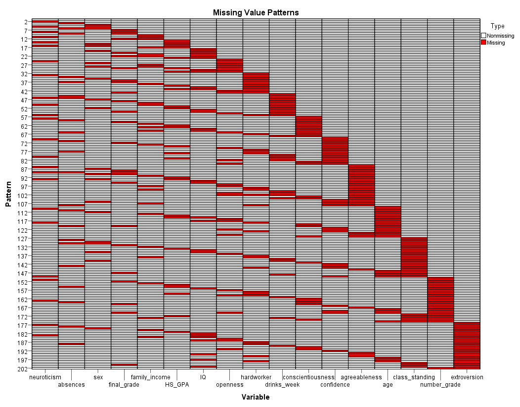
Next, the Missing Value Patterns chart is displayed (it has been grossly enlarged to enhance interpretability). Each pattern (row) reflects a group of cases with the same pattern of missing values; in other words, the patterns or groups of cases are displayed based on where the missing values are located (i.e. on each variable). The variables along the bottom (x-axis) are ordered by the amount of missing values each contains. Consider the table above, neuroticism has the lowest percentage of missing values (3.9%) and is therefore, listed first (on the left), while extroversion which has the largest percentage of missing values (5.4%) is listed last (on the right). For example; the first pattern is always one which contains no missing values. The second pattern reflects only cases with missing values on the neuroticism variable. The chart allows one to assess monotonicity (i.e. rigid decreasing or increasing across a sequence). Essentially if all the missing cells and non-missing cells are touching, then monotonicity is present. Because we have clumps or islands of missing and non-missing cells, we can conclude that this data's missingness does not display monotonicity and therefore, the monotone method of imputation is not justified.

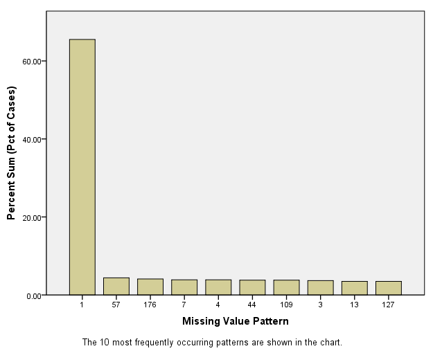
Next, the Pattern Frequencies graph is displayed. This graph shows that the first pattern (one in which no missing values are present) is the most prevalent. The other patterns are much less prevalent, but roughly equally so.

2.) Impute Missing Data Values

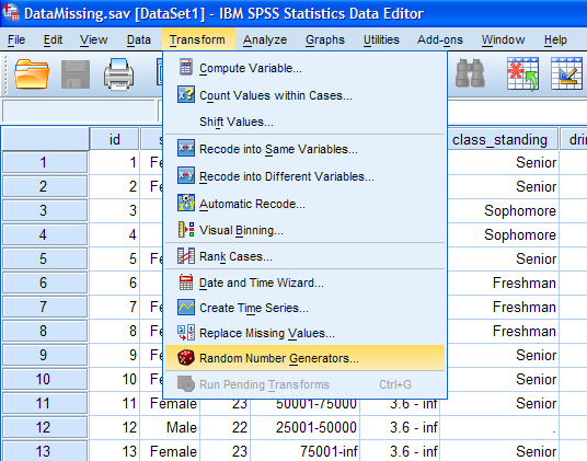
Since we would like to be able to reproduced the results (output below) and multiple imputation is an iterated process (i.e. you can get slightly different results each time it is done), we must first set the random seed. To do this, click on Transform, then Random Number Generators...

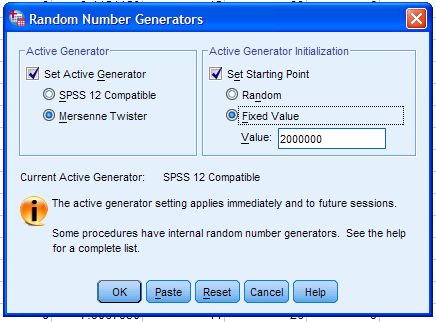
Next, select Set Active Generator, then Mersenne Twister, then select Set Starting Point and Fixed Value. Then, click the OK button.

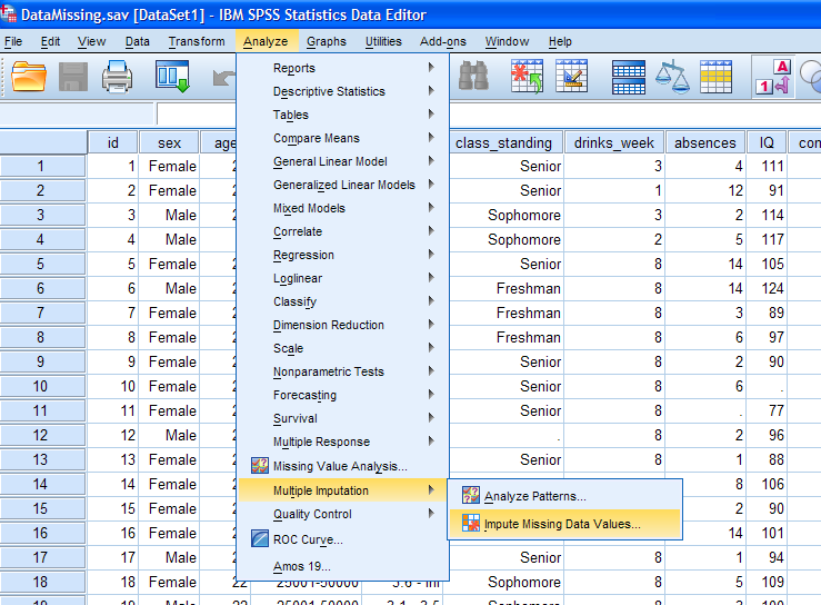
Now we can conduct the multiple imputation. Begin by clicking on Analyze, Multiple Imputation, then Impute Missing Data Values...

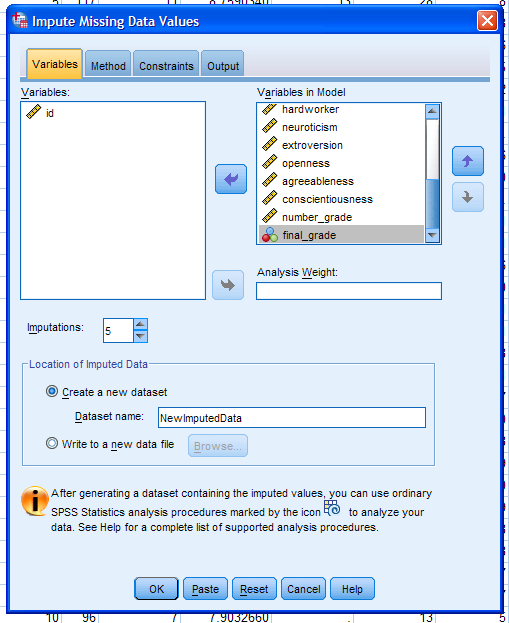
Next, select all the variables (excluding the case identification variable) and move them to the Variables in Model box. Then, click the Create a new dataset circle and type in a name for the imputed data set which will be created. This data set will contain imputed values in place of the missing values. It is important to note that the operation actually does 5 (default, which is fine) imputation runs; meaning five imputations are performed in sequence. During each imputation the missing values are imputed and at the end of the imputations (all 5 in this case), the values are averaged together to take into account the variance of the missing values. This is why the procedure is called multiple imputation; because you end up with one set of imputed values -- but those values are in fact aggregates of multiple imputed values. At the risk of beating a dead horse, imagine that the fourth case is missing the extroversion score. That score will be imputed 5 times and stored in data sets, then those 5 values will be averaged and the resulting (single) value will be used in the primary analysis of the study. Multiple imputation is a strategy or process, there are many methods of going about the process of multiple imputation, such as implementation of the EM algorithm (often referred to as maximum likelihood imputation), but it is not the only method (monotone is also available in the Missing Values module of SPSS, while there are many, many more methods available in R).

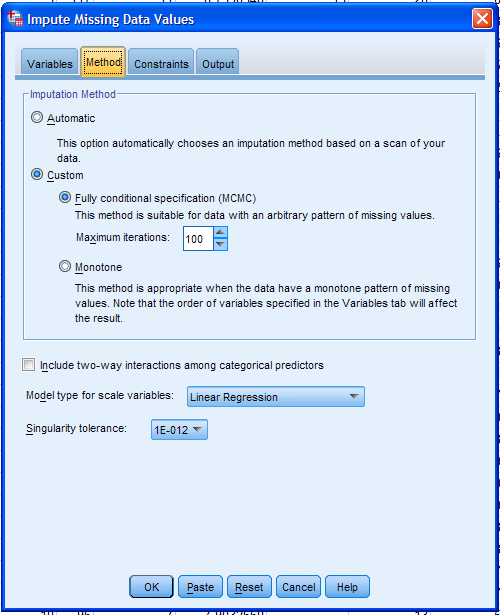
Next, click on the Method tab. There are only two methods available: Markov Chain Monte Carlo method (MCMC) and Monotone. The automatic function scans the data for monotonicity and if discovered uses the Monotone method...otherwise, it defaults to the MCMC method (with 10 iterations and a standard regression model type). Next, up the iterations from 10 (default) to 100 to increase the likelihood of attaining convergence (when the MCMC chain reaches stability -- meaning the estimates are no longer fluctuating more than some arbitrarily small amount). Next, choose the Model type; keeping standard Linear Regression (default). The alternative is Predictive Mean Matching (PMM). PMM still uses regression, but the resulting predicted values are adjusted to match the closest (actual, existing) value in the data (i.e. the nearest non-missing value to the predicted value). If so desired, all possible two-way interactions among categorical predictors can be included in the (regression) model. Next, click the Constraints tab.

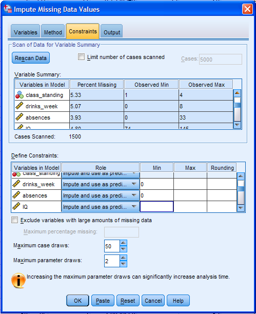
The Constraints tab allows the user to specify a variety of options for the process. First, click the Scan Data button, which will scan the data to fill in the Variable Summary table. This information can be (will be) used in the Define Constraints table. Obviously, for some variables, there are a finite number of valid values (e.g. minimum of zero for drinks_week and absences) and so, we would want to constrain the analysis to those minimum and maximum valid values. Categorical variables are automatically dummy coded; so Min, Max, and Rounding are not necessary. However, specification of the Min, Max, and Rounding can only be done when Linear Regression is specified as the Variable Model. By default all variables will be considered as both predictor and outcome (imputed) during the analysis. However, if for some reason you wanted to set a variable(s) as only a predictor or only a outcome, then the Role column can be used for that purpose. Below the Define Constraints table, one can also specify that variables be excluded from the analysis if they have a maximum (specified) percentage of missing values. Lastly, if Min, Max, and/or Rounding are specified, then the analysis will continue drawing values until those constraints are satisfied or until the Maximum case draws and/or Maximum parameter draws have been reach -- which can be manipulated by the user -- and an error occurs (i.e. the process is not completed). Next, click on the Output tab.

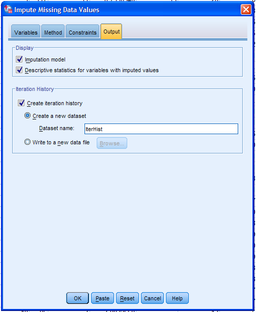
Here, we can specify what is to be displayed in the output window. Select Descriptive statistics for variables with imputed values and Create iteration history; naming the dataset to be created "IterHist". The iteration history is often useful for diagnosing convergence failures or errors (as mentioned above with the maximum case and parameter draws).

Finally, we can click the OK button. [Note, depending on number of iterations and maximum case and parameter draw specifications, the processing time can be quite long.]

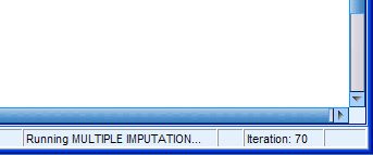
The iteration numbers are listed in the lower right corner of the output window as they occur. Keep in mind, we have specified (above) that 100 iterations should be run for each of the 5 imputations.

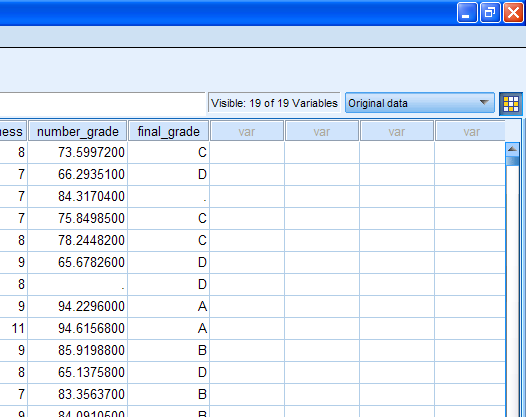
When the process finishes, you should have two new data files (NewImputedData.sav & IterHist.sav) and quite a lot of new output. First, take a look at the imputed dataset. You'll notice there are several subtle differences in the data editor window when compared to the original data (DataMissing.sav). Three things which stand out are the missing values (blank cells), the new variable on the far left side of the data, called "Imputation_", and on the far right (pictured in the second image below) is the little cube of white and yellow cells with a drop-down menu (with "Original data" shown).

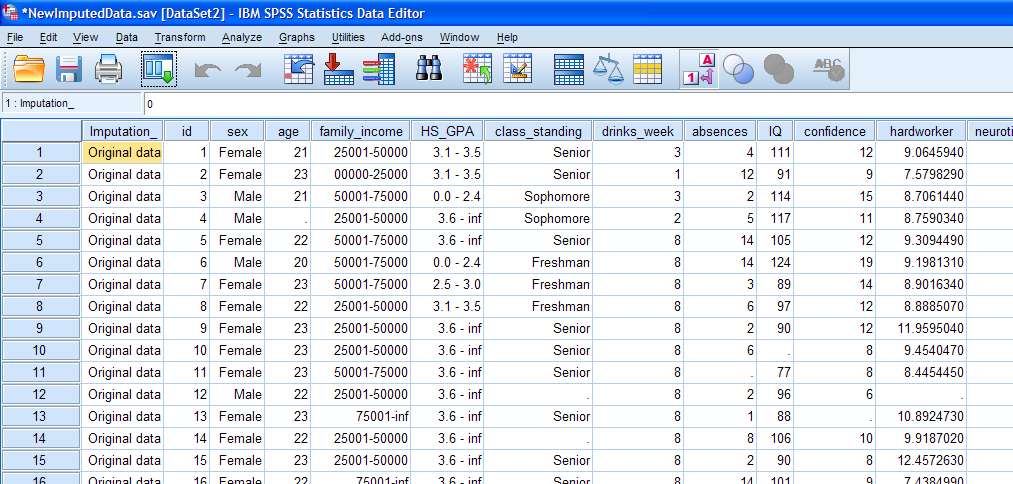
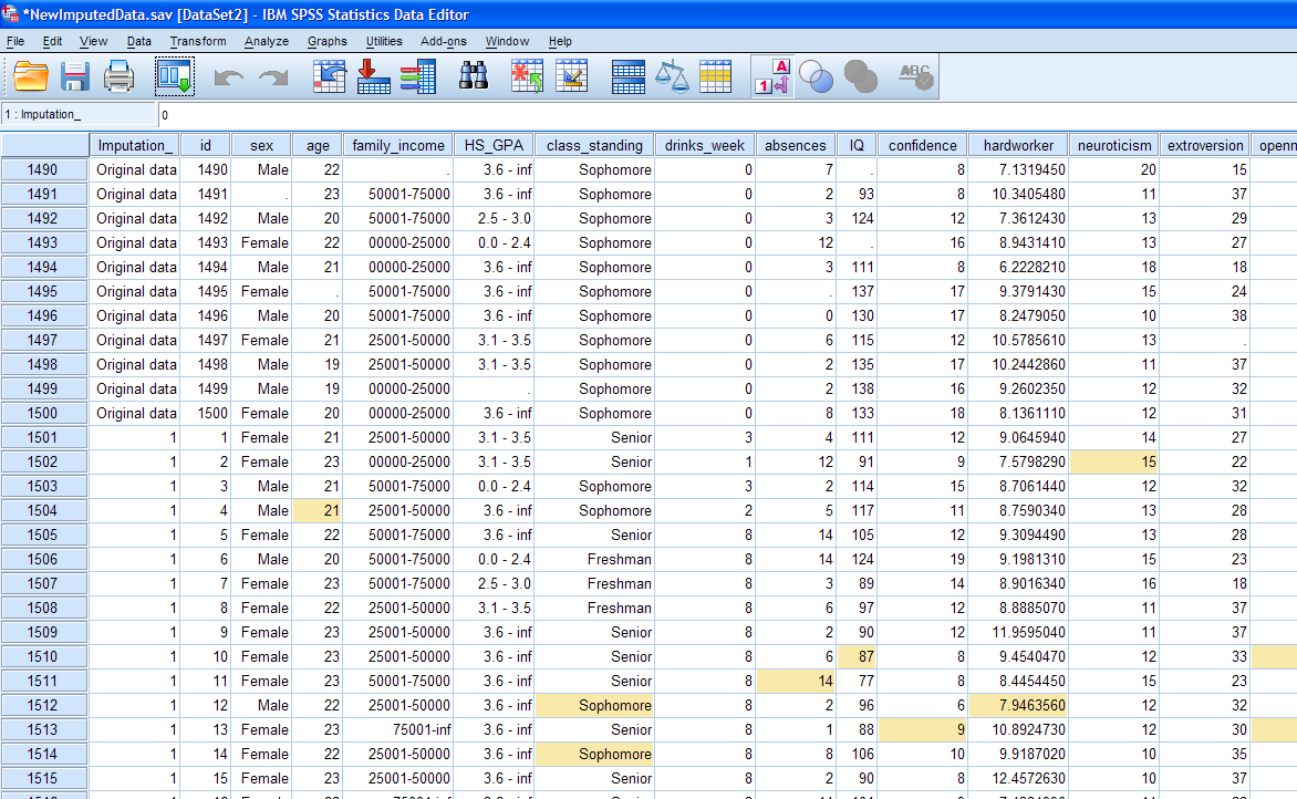
The Imputation variable simply labels each of the imputation sets. The first set is the original data (1500 cases) with the missing values still present. Below it, you'll notice the value for the Imputation_ variable changes to a number "1" (1500 more cases) which shows the first set of imputed; meaning the first of the 5 sets we requested and the other four sets are listed below the original and first sets. You can also use the drop-down menu at the extreme right (shown above) to move between each set. Notice, SPSS marks the cells which contain imputed values by highlighting them (i.e. changing the background of the cells to yellow). The little cube (shown above) which is next to the drop-down menu for moving between imputed sets is colored white and yellow to identify that this data file is an imputed data file. 

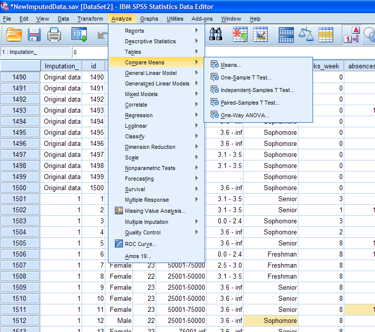
Another very important thing to notice about this imputed data file, which is not readily apparent, is the fact that the Data Editor is aware that this file is an imputed data file. As such, if you click on Analyze, then some analysis (e.g. Compare Means), you'll notice that many of the analyses are compatible with imputed data. In other words, each analysis or function which shows an icon (shown below), which looks like the cube with a concentric swirl next to it, will automatically be run on the aggregated imputed data ("pooled" estimates).

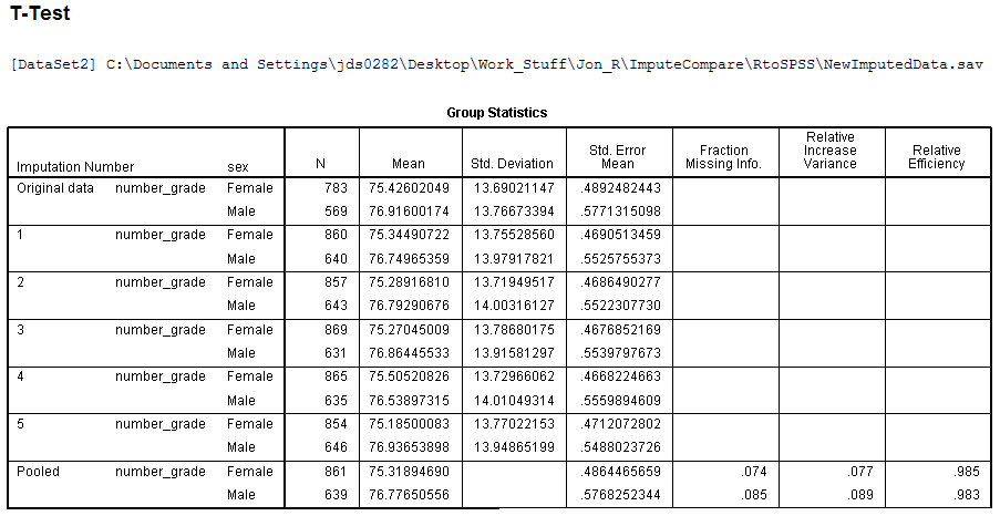
As a quick example of pooled output, if we run a simple independent samples t-test comparing males and females on number grade, we get the following output -- which displays results for (1) the original data (with missing), (2) each imputation set separately, and (3) the 'pooled' estimates. [Note: only the Group Statistics table is shown, the second table (t-test results table) is not shown.]

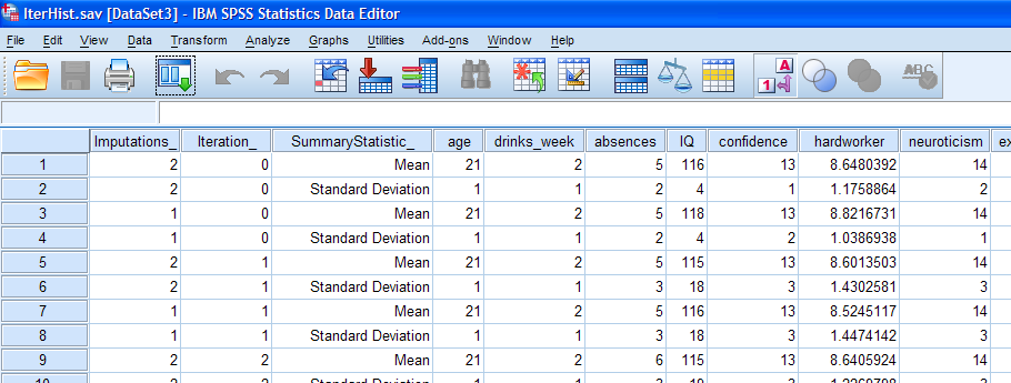
The second data set produced by the imputation process is the iteration history data set (IterHist.sav). This file simply lists the mean and standard deviation for each interval/ratio scaled variable by iteration and imputation. By plotting the mean and standard deviation of a particular variable across iterations and imputations, one can assess the patterns of the imputed values. These plots should show a fairly random pattern (i.e. no discernable pattern).

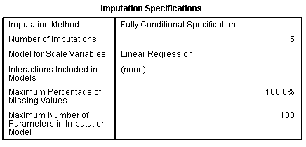
Next, we can review the output created by the imputation process.

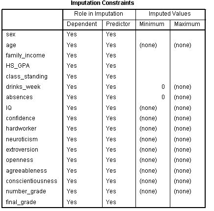
The first table, Imputation Specifications, simply lists what was specified for the process. The second table, Imputation Constraints, again simply lists what was specified on the Constraints tab prior to running the process.

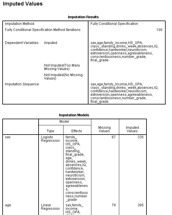
The next two tables, Imputation Results and Imputation Models, simply display what occurred during the imputation procedure. [Note: The majority of the second table (Imputation Models) is not displayed.]

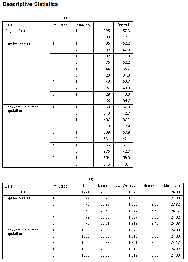
The next section of output contains one table for each variable, displaying descriptive statistics for each variable in the original data (with missing) and at each imputation for both the (specific) imputed values and (globally) all the values (i.e. all cases after imputation) of the variable. [Note: Only the sex variable and the age variables' tables are shown.]

And that's it. As mentioned above, many analyses in SPSS (here version 19) are able to consider imputed data sets and offer pooled output (i.e. showing the results of the analysis for each imputation set, as was done above with the quick t-test example). For a complete list of the analyses capable of utilizing imputed data, refer to the module's manual (specifically pages 29 - 31).

 IBM (2010). IBM SPSS Missing Values 19: User's Guide. Available at:

Return to the SPSS Short Course