|
Categorical Regression (CATREG)
The SPSS CATREG function incorporates optimal
scaling and can be used when the predictor(s) and outcome variables are
any combination of numeric, ordinal, or nominal. Standard multiple
regression can only accommodate an outcome variable which is continuous
or nearly continuous (i.e. interval/ratio in scale) and it works best
with continuous or nearly continuous predictor variables. Although
standard regression can accommodate categorical predictors using one of
the following strategies for those types of predictors: dummy coding,
effects coding, orthogonal coding, or criterion coding. Binomial
Logistic regression is appropriate when the outcome is a dichotomous
variable (i.e. categorical with only two categories). Multi-nomial
Logistic Regression or Discriminant Function Analysis is appropriate
when the outcome variable is polytomous (i.e. categorical with more
than two categories).
It is recommended that when conducting categorical regression, one
approach the process as one would approach a data reduction process;
meaning it is often necessary to conduct multiple runs of the analysis
while slightly changing the options / parameters in an effort to
discover the best results (i.e. best fitting model and most
substantively meaningful interpretation of results).
For the duration of this tutorial we will be using
the
SPSScatreg.sav
file; which contains 1 outcome variable (y) and 5 predictor variables
(x1 - x5). The outcome variable was operationally defined as general
happiness and was measured with a subjective rating scale. Each of the
five predictors were 8-point Likert scaled questionnaire items which
are believed to measure preferences for various types of social
interactions.
(1) Evaluate the variables.
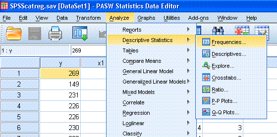
Begin by conducting a Frequency function to get an
idea of how our variables are distributed. Click on Analyze,
Descriptive Statistics, Frequencies...
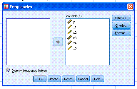
Next, highlight / select all of the variables and
use the arrow button to move them to the Variable(s): box. Then click
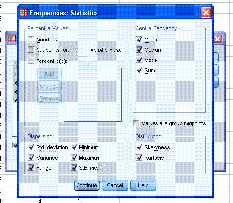
on the Statistics... button and select the following. Then click
Continue.
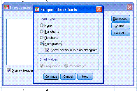
Next, click on the Charts... button, and select,
Histograms: and then click the box for Show normal curve on histogram.
Then click the Continue button, then click the OK button.
The output should be similar to what is displayed
below.
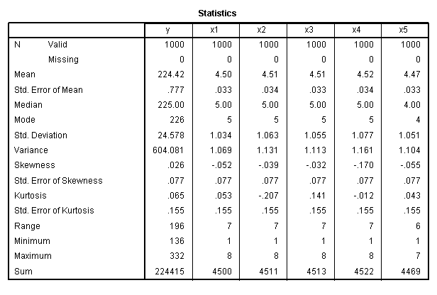
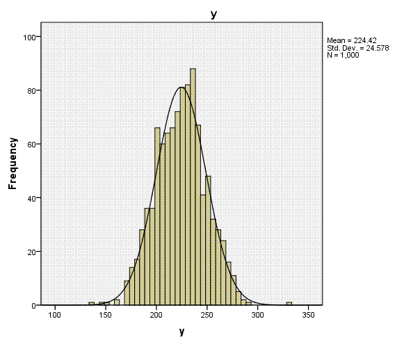
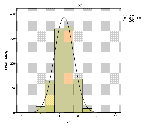
Here, we see that our outcome variable not only
has a substantial range of 196 values, but it also has very low values
for skewness (.026) and kurtosis (.065) which indicate a fairly
normally distributed variable. In fact, we could treat this ordinal
variable as numeric or nearly continuous and decide to run a standard
multiple regression. But, we would need to use a coding strategy
for the predictor variables if we did choose to run the
standard multiple regression. Also, as this example shows, it is better
to run a categorical regression on this data because of the opportunity
to apply optimal scaling and because all the predictors appear to be
and are nominal or ordinal.
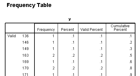
The frequency table for y has been truncated to
save space, but it too shows how broadly distributed the values are on
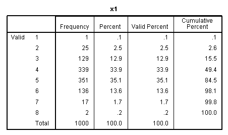
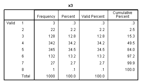
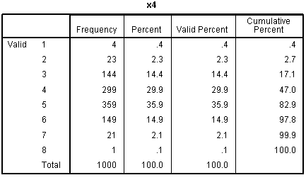
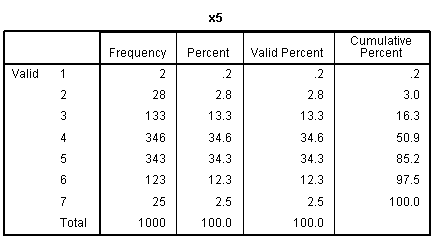
our outcome variable. The other frequency tables show the discrete
nature of our predictor variables.

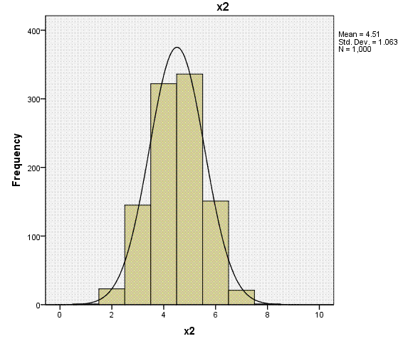
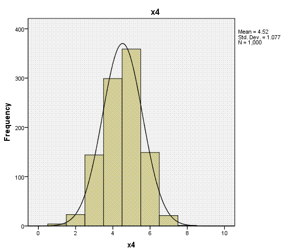
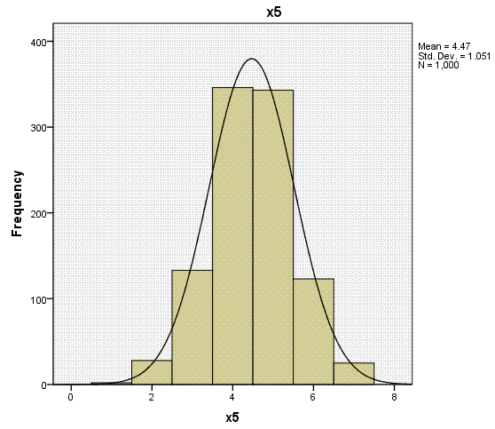
Again, the histogram (with super-imposed normal
curves) shows how well our outcome variable (which is nominal) displays
the characteristics of an interval or ratio variable. Bar charts would
be more appropriate for categorical variables (showing the discrete
nature of the variables), but we can see each of the predictors
displays narrow range across values 1 - 8.

(2) Standard (multiple) Regression for
comparison.
Running a standard multiple regression gives us a
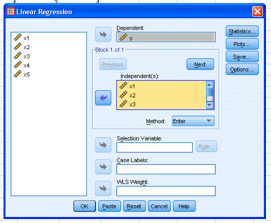
baseline model for comparison. Click on Analyze, Regression, Linear...
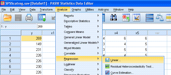
Next, highlight / select y and use the top arrow
button to move it to the Dependent: box. Then, select all the
predictors and move them to the Independent(s): box. Then, click the
Statistics button.
 Next, select Descriptives (this will produce a Pearson correlation
matrix).
Next, select Descriptives (this will produce a Pearson correlation
matrix).
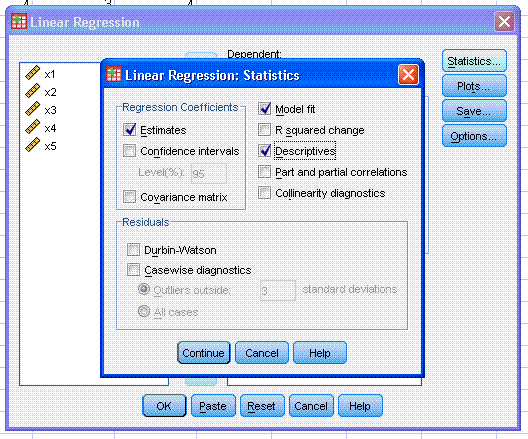
Next, click the Continue button, then click the OK
button.
The output should be similar to what is displayed
below.
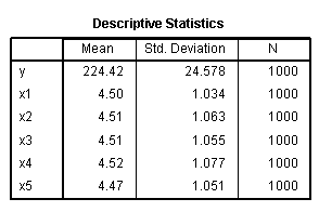
The Descriptive Statistics table shows some of the
same information provided in the frequencies function above. The
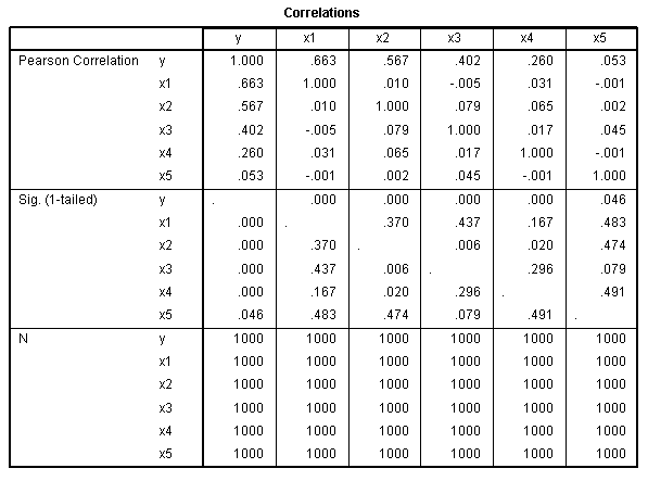
Correlations table provides us with an idea of the relationship between
each of the variable. It provides only an idea, because a polychoric
correlation matrix (rather than a Pearson correlation matrix) would be
more appropriate given the nature of the variables. Pay particular
attention to the relationships between each predictor and the outcome
variable. Also, notice the lack of multicollinearity (i.e. low
magnitude relationships between the predictors). The significance
associated with this data is likely to be of little use given the
fairly large sample size of the data (N = 1000).
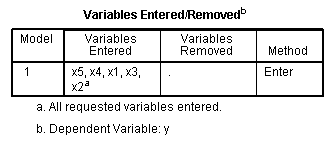
The Variables Entered/Removed table shows just
that, all the predictors in the model and none removed. The Model
Summary tables shows the multiple correlation coefficient (R?), squared multiple
correlation coefficient (R?), adjusted multiple
correlation coefficient (adj.R?), and standard error
of the estimate. According to our model summary, the collection of
predictors accounts for 92.6% (adj.R? = .926) of the
variance in our outcome variable.

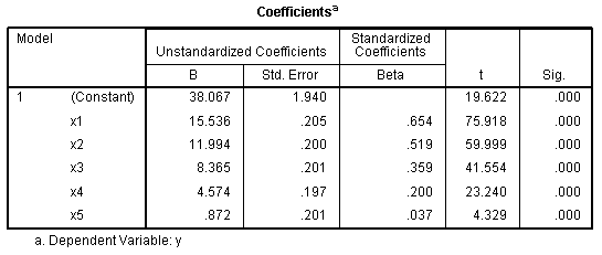
The ANOVA table simply tells us our R? is significantly different from
zero. Pay particular attention to the magnitude and order of magnitude
of the standardized coefficients or Beta (β)coefficients, for each of
our predictors in the Coefficients table. They should be close to the
bi-variate correlations for each predictor with the outcome, as listed
above in the Correlations table.

(3) First Categorical Regression
Analysis.
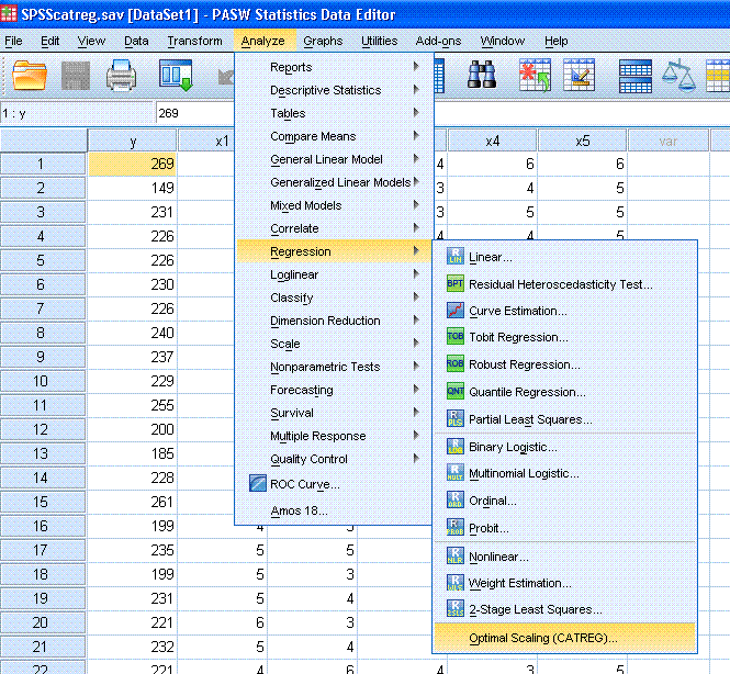
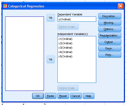
Returning to the Data Window, click on Analyze,
Regression, Optimal Scaling (CATREG)...
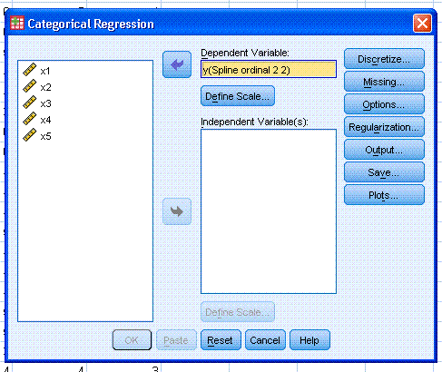
Next, select the outcome variable (y) and use the
top arrow button to move it to the Dependent Variable: box. Then, click
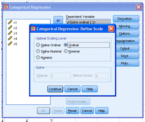
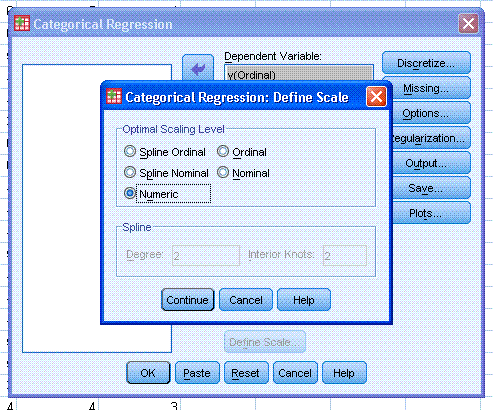
on the top Define Scale... button and select Ordinal. You can see here
the different levels of scale / measurement available. Then, click the
Continue button.
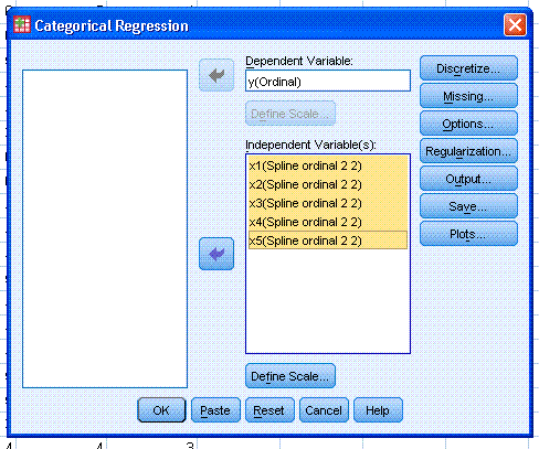
Next, select all 5 predictor variables and use the
lower arrow button to move them to the Independent Variable(s): box.
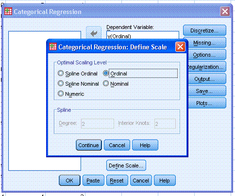
Then, click on the lower Define Scale... button and select Ordinal for
all 5 predictors. Again, you can see here the different levels of scale
/ measurement available. Then, click the Continue button.
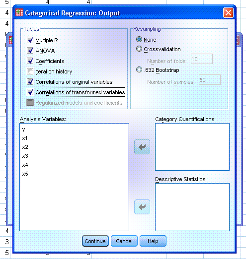
Next, click on the Output... button and select
Correlations of original variables and Correlations of transformed
variables. Then click the Continue button. Notice, if you click on the
Save... button, you have the ability to save predicted and / or
residual values. Next, click the OK button. Keep in mind, the optimal
scaling process is iterative and can take a minute or more.
The output should be similar to what is displayed
below.
The first two tables are of little to no interest
for interpretation; we now know who to thank for inclusion of this
analysis in SPSS and there was no missing data.

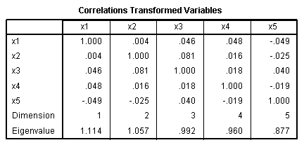
The two correlation tables show the original
relationships between the predictor variables (identical to what we saw
in the original Correlations table above), and the correlations between
our transformed (i.e. optimally scaled) predictor variables. Again,
there is no danger of violating the regression assumption of no
multicollinearity; meaning, our predictor variables are not
substantially related.

The Model Summary table shows an unrealistic
multiple correlation coefficient. Regression assumes correct model
specification (i.e. all important variables in the model and no
un-important variables in the model); so given the simulated nature of
this data, it is reporting perfect fit because, all of the important
variables are in the model --
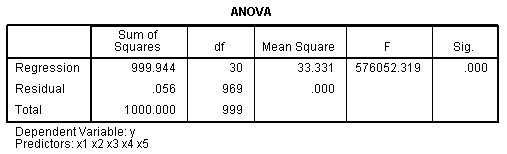
which never happens with 'real' data. Of course, the ANOVA table is
showing that our R?
value is significantly different from zero. The R script file used to
generate this data can be found
here.

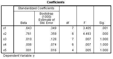
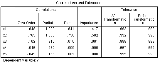
The Coefficients table and the Correlations and
Tolerance table display a rather curious pattern of relationships
between each predictor and the outcome when compared to the
correlations and Beta coefficients tables displayed in the standard
multiple regression. Focus on the Beta coefficients, zero-order
correlations, partial correlations, part correlations (semi-partial),
and importance. In these two tables, the strongest predictor is x2; and
x3, x4, x5 are not significant predictors of y. It seems as though the
CATREG algorithm is confusing the importance of x1 & x2,
inflating the importance of x2, and completely discounting the
importance of x3, x4, & x5.
In pursuit of a more clear and realistic
interpretation for this data and the relationships between the
variables, we can run a second CATREG with the outcome variable
specified as numeric.
(4) Second Categorical Regression
Analysis.
Returning to the Data Window, click on Analyze,
Regression, Optimal Scaling (CATREG)...
You'll notice the previous run of the analysis is
still specified. Here, all we need to do is highlight / select y in the
Dependent Variable: box, then click on the Define Scale... button
(marked here with a red ellipse).
Next, change the scale from Ordinal to Numeric.
Then click the Continue button, then click the OK button.
The output should be similar to what is displayed
below.
The first two tables are identical to those from
the previous run.
The Correlations Original Variables table is
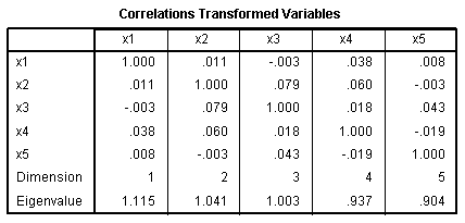
identical to the previous run. The correlations between our transformed
(i.e. optimally scaled) predictor variables have changed because of the
(newly produced) iterative optimally scaled data. Again, there is no
danger of violating the regression assumption of no multicollinearity.
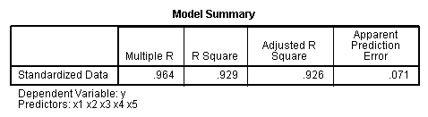
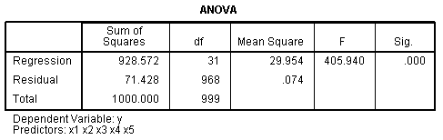
The Model Summary table offers more realistic
representations of the multiple correlation between all 5 predictors
and our outcome variable. The ANOVA table again shows that our R? is significantly
different from zero.
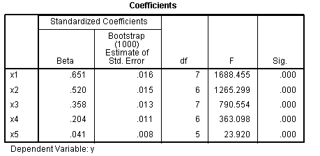
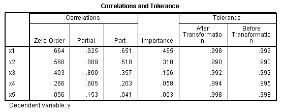
The Coefficients table (Beta coefficients) and the
Correlations and Tolerance table (zero-order correlations, partial
correlations, part correlations (semi-partial), & importance)
shows values which more closely resemble the original relationships.
This should highlight the importance of (1) knowing the operational
definitions of variables, (2) conducting initial data analysis (IDA) by
running frequencies and / or descriptive statistics functions, and (3)
conducting multiple analysis while modifying the options / parameters
to extract as much information as possible from the data. Here, the
true relationships of the variables are reflected while running the
appropriate analysis for the measurement scale of the variables. In
this example we knew the true relationships between the variables
because we used simulation to generate the data. In a genuine research
study, it is recommended one conduct simulation studies in order to
more easily recognize the patterns in the data and have confidence in
the analysis being performed. However, even if simulation is not used
prior to collecting the actual data, one should have at least some
understanding of the underlying relationships between the variables of
interest based on a thorough literature review (i.e. prior research and
theory associated with the area of study).
REFERENCES and RESOURCES
de Leeuw, J. (1988). Multivariate analysis with
linearizable regressions.
Psychometrika, 53(4), 437 - 454. (here).
Meulman, J. J. (1998). Optimal scaling
methods for multivariate categorical data analysis. SPSS
White Paper, SPSS Inc. (here).
SPSS Content Guideline for CATREG in PASW 18. (here).
Van Der Geer, J. P. (1993). Multivariate analysis
of categorical data: Theory. Advanced Quantitative Techniques in the
Social Sciences Series (Vol. 2). Sage Publications, Inc.
Van Der Geer, J. P. (1993). Multivariate analysis
of categorical data: Applications. Advanced Quantitative Techniques in
the Social Sciences Series (Vol. 3). Sage Publications, Inc.
|