|
Factor
Analysis
with Maximum Likelihood Extraction in SPSS.
Before we begin with the analysis; let's take a
moment to address and hopefully clarify one of the most confusing and
misarticulated issues in statistical teaching and practice
literature.
First, Principal Components Analysis (PCA)
is a variable reduction technique which maximizes the amount of
variance accounted for in the observed variables by a smaller group of
variables called COMPONENTS. As an example, consider the following
situation. Let's say, we have 500 questions on a survey we designed to
measure persistence. We want to reduce the number of questions so that
it does not take someone 3 hours to complete the survey. It would be
appropriate to use PCA to reduce the number of questions by identifying
and removing redundant questions. For instance, if question 122 and
question 356 are virtually identical (i.e. they ask the exact same
thing but in different ways), then one of them is not necessary. The
PCA process allows us to reduce the number of questions or variables
down to their PRINCIPAL COMPONENTS.
PCA is commonly, but very confusingly, called
exploratory factor analysis (EFA). The use of the word factor
in EFA is inappropriate and confusing because we are really interested
in COMPONENTS, not factors. This issue is made more confusing by some
software packages (e.g. PASW/SPSS & SAS) which list or use PCA
under the heading factor analysis.
Second, Factor Analysis (FA) is
typically used to confirm the latent factor structure for a group of
measured variables. Latent factors are unobserved variables which
typically can not be directly measured; but, they are assumed to cause
the scores we observe on the measured or indicator variables. FA is a
model based technique. It is concerned with modeling the relationships
between measured variables, latent factors, and error.
As stated in O'Rourke, Hatcher, and Stepanski
(2005): "Both (PCA & FA) are methods that can be used to
identify groups of observed variables that tend to hang together
empirically. Both procedures can also be performed with the SAS FACTOR
procedure and they generally tend to provide similar results.
Nonetheless, there are some important conceptual differences between
principal component analysis and factor analysis that should be
understood at the outset. Perhaps the most important deals with the
assumption of an underlying causal structure. Factor analysis assumes
that the covariation in the observed variables is due to the presence
of one or more latent variables (factors) that exert causal influence
on these observed variables" (p. 436).
Final thoughts. Both PCA and FA can be used as
exploratory analysis. But; PCA is predominantly used in an exploratory
fashion and almost never used in a confirmatory fashion. FA can be used
in an exploratory fashion, but most of the time it is used in a
confirmatory fashion because it is concerned with modeling factor
structure. The choice of which is used should be driven by the goals of
the analyst. If you are interested in reducing the observed variables
down to their principal components while maximizing the variance
accounted for in the variables by the components, then you should be
using PCA. If you are concerned with modeling the latent factors (and
their relationships) which cause the scores on your observed variables,
then you should be using FA.
O'Rourke, N., Hatcher, L., & Stepanski,
E.J. (2005). A step-by-step approach to using SAS for univariate and
multivariate statistics, Second Edition. Cary, NC: SAS Institute Inc.
Factor Analysis
The following covers a few of the SPSS procedures
for conducting factor analysis with maximum likelihood extraction. For
the duration of this tutorial we will be using the
ExampleData4.sav
file.
FA 1. Begin by clicking on
Analyze, Dimension Reduction, Factor...

Next, highlight all the variables of interest (y1
- y15) and use the top arrow button to move them to the Variables: box.
Then click the Descriptives button and select the following. Then click
the Continue button.

Next, click on the Extraction button. In the
Method drop-down menu, choose Maximum likelihood. Then select Unrotated
factor solution and Scree plot. Notice the extraction is based on
factors with eigenvalues greater than 1 (by default). There are a
number of perspectives on determining the number of factors to extract
and what criteria to use for extraction. Originally, eigenvalues
greater than 1 was generally accepted. However, more recently
Zwick
and Velicer (1986) have suggested, Horn’s (1965) parallel analysis
tends to be more precise in determining the number of reliable
components or factors. Unfortunately, Parallel Analysis is not
available in SPSS. Therefore, a review of the parallel analysis engine (Patil, Singh, Mishra,
& Donavan, 2007) is strongly recommended. Next,
click the Continue button.
 Next,
click on Scores and select Save as Variables. This will create new
variables (1 per extracted factor) which will allow us to evaluate
which type of rotation strategy is appropriate in subsequent factor
analysis. Next,
click on Scores and select Save as Variables. This will create new
variables (1 per extracted factor) which will allow us to evaluate
which type of rotation strategy is appropriate in subsequent factor
analysis.

Next, click the OK button.
The output should be similar to that displayed
below.
The Descriptive Statistics table simply provides
mean, standard deviation, and number of observations for each variable
included in the analysis.
The Correlation Matrix table provides correlation
coefficients and p-values for each pair of variables included in the
analysis. A close inspection of these correlations can offer insights
into the factor structure.

 The next
table is used as to test assumptions; essentially, the
Kaiser-Meyer-Olking (KMO) statistic should be greater than 0.600 and
the Bartlett's test should be significant (e.g. p <
.05). KMO is used for assessing sampling adequacy and evaluates the
correlations and partial correlations to determine if the data are
likely to coalesce on factors (i.e. some items highly correlated, some
not). The Bartlett's test evaluates whether or not our correlation
matrix is an identity matrix (1 on the diagonal & 0 on the
off-diagonal). Here, it indicates that our correlation matrix (of
items) is not an identity matrix--we can verify this by looking at the
correlation matrix. The off-diagonal values of our correlation matrix
are NOT zeros, therefore the matrix is NOT an identity matrix. The next
table is used as to test assumptions; essentially, the
Kaiser-Meyer-Olking (KMO) statistic should be greater than 0.600 and
the Bartlett's test should be significant (e.g. p <
.05). KMO is used for assessing sampling adequacy and evaluates the
correlations and partial correlations to determine if the data are
likely to coalesce on factors (i.e. some items highly correlated, some
not). The Bartlett's test evaluates whether or not our correlation
matrix is an identity matrix (1 on the diagonal & 0 on the
off-diagonal). Here, it indicates that our correlation matrix (of
items) is not an identity matrix--we can verify this by looking at the
correlation matrix. The off-diagonal values of our correlation matrix
are NOT zeros, therefore the matrix is NOT an identity matrix.
 A
communality (h?)
is the sum of the squared factor loadings and represents the amount of
variance in that variable accounted for by all the factors. For
example, all five extracted factors account for
33.4% of the variance in variable y1 (h? = .334). A
communality (h?)
is the sum of the squared factor loadings and represents the amount of
variance in that variable accounted for by all the factors. For
example, all five extracted factors account for
33.4% of the variance in variable y1 (h? = .334).
The next table displays the amount of variance
accounted for in the variables' or items' variance-covariance matrix by
each of the factors and cumulatively by all the factors. Here we see
that all 5 extracted factors (those with an eigenvalue greater than 1)
account for 32.209% of the variance in the items' variance-covariance
matrix.
The scree plot graphically displays the
information in the previous table; the factors' eigenvalues.

The next table displays each variable's loading on
each factor. We notice from the output, we have two items (y14
& y15) which do not load on the first factor (always the
strongest without rotation) but create their own retained factor (also
with eigenvalue greater than 1). We know a factor should have, as a
minimum, 3 items/variables; but let's reserve deletion of items until
we can discover whether or not our factors are related.
Finally, we have the goodness-of-fit table; which
gives an indication of how well our 5 factors reproduce the variables'
or items' variance-covariance matrix. Here, the test shows that the
reproduced matrix is NOT significantly different from the observed
matrix -- which is what we would hope to find; indicating good
fit.

Next, we will use the saved factor scores to
determine if our factors are correlated, which would suggest an oblique
rotation strategy would be appropriate. If the factors are not
correlated, then an orthogonal rotation strategy is appropriate. Keep
in mind, if literature and theory suggest the factors are related then
you may use an oblique rotation, regardless of what you find in your
data.
In the Data Window, click on Analyze, Correlated,
Bivariate...
Next, highlight and use the arrow button to move
all the REGR factor scores to the Variables: box. Then click the OK
button.

The output should display the correlation matrix
for the 5 factor scores as below.
Here, we see that none of the factor scores are
related, which suggests the factors themselves are not related -- which
indicates we should use an orthogonal rotation in subsequent factor
analysis.
FA 2.
VARIMAX rotation imposed. Next, we re-run the
FA specifying 5 factors to be retained. We will also specify the
VARIMAX rotation strategy, which is a form of orthogonal rotation.
Begin by clicking on Analyze, Dimension
Reduction, Factor...
Next, you should see that the previous run is
still specified; variables y1 through y15. Next click on
Descriptives...and select the following; we no longer need the
univariate descriptives, the correlation matrix, or the KMO and
Bartlett's tests. Then click the Continue button. Next, click on the
Extraction... button. We no longer need the scree plot; but we do need
to change the number of factors to extract. We know from the
first run, there were 5 factors with eigenvalues greater than one, so
we select 5 factors to extract. Then click the Continue button.
Next, click on Rotation... and select Varimax.
Then click the Continue button. Then click on the Scores... button and
remove the selection for Save as Variables. Then click the Continue
button. Then click the OK button.

The first 3 tables in the output should be
identical to what is displayed above from FA 1; accept, now we have two
new tables at the bottom of the output.
The rotated factor matrix table shows which
items/variables load on which factors after rotation. We see that the
rotation cleaned up the interpretation by eliminating the global first
factor. This provides a clear depiction of our
factor structure
(marked with red ellipses).
Again, the Factor Transformation Matrix simply
displays the factor correlation matrix prior to and after
rotation.
FA 3.
Finally, we can eliminate the two items (y14 & y15) which (a)
by themselves create a factor (factors should have more than 2 items or
variables) and (b) do not load on the un-rotated or initial factor 1.
Again, click on Analyze, Dimension Reduction, then Factor...
Again, you'll notice the previous run is still
specified, however we need to remove the y14 and y15 variables. Next,
click on Extraction... and change the number of factors to extract from
5 to 4. Then click the Continue button and then click the OK button.
The output should be similar to what is displayed
below.
 The communalities are lower
than we would prefer (generally would like to see at least 0.450). The communalities are lower
than we would prefer (generally would like to see at least 0.450).
The four extracted (and rotated) factors account
for 35.483 % of the variance in the items' variance-covariance matrix.
The Factor Matrix table displays factor loadings
for each item (prior to rotation).
The goodness-of-fit table; which gives an
indication of how well our 5 factors reproduce the variables' or items'
variance-covariance matrix. Here, the test shows that the reproduced
matrix is NOT significantly different from the observed matrix -- which
is what we would hope to find; indicating good fit.
The Rotated Factor Matrix displays the loadings
for each item on each rotated factor, again clearly showing the factor
structure.

And again, the Factor Transformation Matrix
displays the correlations among the factors prior to and after
rotation.

As a general conclusion, we can say we have four
factors accounting for 35.483 % of the variance in our 13 items. In the
Rotated Factor Matrix table we see clear factor structure displayed;
meaning, each item loads predominantly on one factor. For instance, the
first four items load virtually exclusively on Factor 1. Furthermore,
if we look at the communalities we see that all the items displayed a
communality of 0.30 or greater, with one exception. The exception is
y4, which is a little lower than we would like and given that Factor 1
has three other items which load substantially on it, we may choose to
remove item y4 from further analysis or measurement in the future.
o
= T + e
obs
= True + err
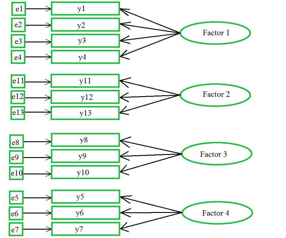
It is important to note that traditional factor
analysis assumes the Classical Test Theory of measurement, which states
that observed scores (obs) are a result of true
scores (True) and error (err).
Therefore, in most factor model diagrams, the arrows point to the
observed variables (note, in the diagram below the coefficients are not
present) reflecting the assumption that the true value of the factor
and the error combines to result in the observed score(s).
REFERENCES / RESOURCES
Horn,
J. (1965). A rationale and test for the number of factors in factor
analysis. Psychometrika, 30, 179 – 185.
O'Rourke, N., Hatcher, L., & Stepanski,
E.J. (2005). A step-by-step approach to using SAS for univariate and
multivariate statistics, Second Edition. Cary, NC: SAS Institute Inc.
Patil,
V. H.,
Singh, S. N., Mishra, S., &
Donavan, D. T. (2007). Parallel Analysis Engine to Aid Determining
Number of Factors to Retain [Computer software]. Retrieved 08/23/2009
from
http://ires.ku.edu/~smishra/parallelengine.htm
Zwick,
W. R., & Velicer, W. F. (1986). Factors influencing five rules
for determing the number of components to retain. Psychological
Bulletin, 99, 432 – 442.
|