MODULE 9

1. Mixed Effects Models

Mixed effects models refer to a variety of models which have as a key feature both fixed and random effects.

The distinction between fixed and random effects is a murky one. As pointed out by Gelman (2005), there are several, often conflicting, definitions of fixed effects as well as definitions of random effects. Gelman offers a fairly intuitive solution in the form of renaming fixed effects and random effects and providing his own clear definitions of each. “We define effects (or coefficients) in a multilevel model as constant if they are identical for all groups in a population and varying if they are allowed to differ from group to group” (Gelman, p. 21). Other ways of thinking about fixed and random effects, which may be useful but are not always consistent with one another or those given by Gelman above, are discussed in the next paragraph.

Fixed effects are ones in which the possible values of the variable are fixed. Random effects refer to variables in which the set of potential outcomes can change. Stated in terms of populations, fixed effects can be thought of as effects for which the population elements are fixed. Cases or individuals do not move into or out of the population. Random effects can be thought of as effects for which the population elements are changing or can change (i.e. random variable). Cases or individuals can and do move into and out of the population. Another way of thinking about the distinction between fixed and random effects is at the observation level. Fixed effects assume scores or observations are independent while random effects assume some type of relationship exists between some scores or observations. For instance, it can be said that gender is a fixed effect variable because we know all the values of that variable (male & female) and those values are independent of one another (mutually exclusive); and they (typically) do not change. A variable such as high school class has random effects because we can only sample some of the classes which exist; not to mention, students move into and out of those classes each year.

There are many types of random effects, such as repeated measures of the same individuals; where the scores at each time of measure constitute samples from the same participants among a virtually infinite (and possibly random) number of times of measure from those participants. Another example of a random effect can be seen in nested designs, where for example; achievement scores of students are nested within classes and those classes are nested within schools. That would be an example of a hierarchical design structure with a random effect for scores nested within classes and a second random effect for classes nested within schools. The nested data structure assumes a relationship among groups such that members of a class are thought to be similar to others in their class in such a way as to distinguish them from members of other classes and members of a school are thought to be similar to others in their school in such a way as to distinguish them from members of other schools. The example used below deals with a similar design which focuses on multiple fixed effects and a single nested random effect.

2. Linear Mixed Effects Models

Linear mixed effects models simply model the fixed and random effects as having a linear form. Similar to the General Linear Model, an outcome variable is contributed to by additive fixed and random effects (as well as an error term). Using the familiar notation, the linear mixed effect model takes the form: 

y_ij = β₁x_1ij + β₂x_2ij … β_nx_nij + b_i1z_1ij + b_i2z_2ij … b_inz_nij + ε_ij

where y_ij is the value of the outcome variable for a particular ij case, β₁ through β_n are the fixed effect coefficients (like regression coefficients), x_1ij through x_nij are the fixed effect variables (predictors) for observation j in group i (usually the first is reserved for the intercept/constant; x_1ij = 1), b_i1 through b_in are the random effect coefficients which are assumed to be multivariate normally distributed, z_1ij through z_nij are the random effect variables (predictors), and  ε_ij is the error for case j in group i where each group’s error is assumed to be multivariate normally distributed.     

3. Example Data

The example used for this tutorial is fictional data where the interval scaled outcome variable Extroversion (extro) is predicted by fixed effects for the interval scaled predictor Openness to new experiences (open), the interval scaled predictor Agreeableness (agree), the interval scaled predictor Social engagement (social), and the nominal scaled predictor Class (classRC); as well as the random (nested) effect of Class (classRC) within School (schoolRC) as well as the random effect of School (schoolRC). The data contains 1200 cases evenly distributed among 24 nested groups (4 classes within 6 schools). The data set is available here.

4. Running the Analysis

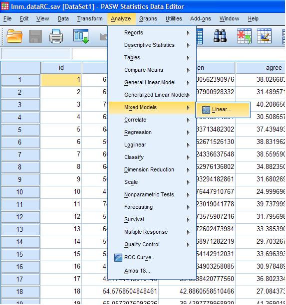
Begin by clicking on Analyze, Mixed Models, Linear...

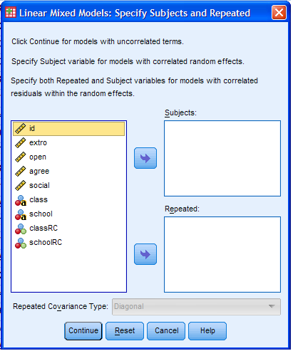
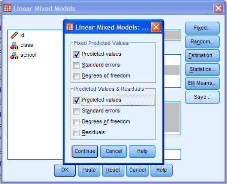
The initial dialogue box is self-explanatory; but will not be used in this example so click the Continue button.

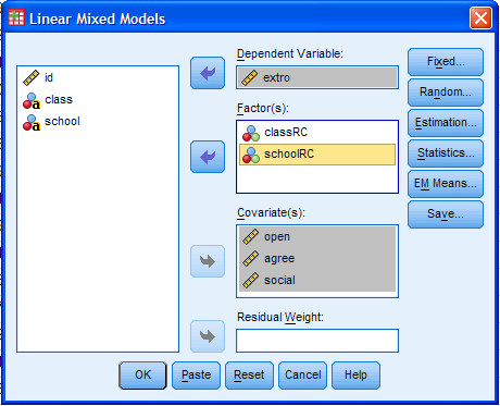
Next, we have the main Linear Mixed Models dialogue box. Here we specify the variables we want included in the model. Using the arrows; move extro to the Dependent Variable box, move classRC and schoolRC to the Factor(s) box, and move open, agree, and social to the Covariat(s) box. Then click on the Fixed... button to specify the fixed effects.

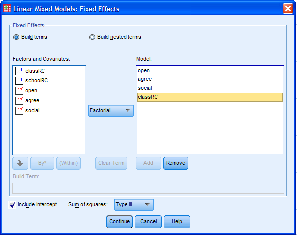
The fixed effects in a LINEAR mixed effects model are essentially the same as a traditional ordinary least squares linear regression. To specify the fixed effects, use the Add button to move open, agree, social, and classRC into the Model box. Notice we are not specifying any interaction terms for this model. Then click the Continue button.

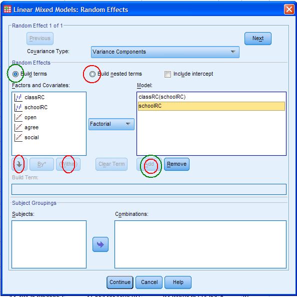
Next, click on the Random... button to specify the random effects.

The first thing we need to do is click on the Build nested terms circle (marked with the top, centered red ellipse). Then, highlight / select the classRC factor and use the down arrow button (marked with the lower, left red ellipse) to move classRC into the Build Term box. Then click the (Within) button (marked with the lower, middle ellipse). Next, highlight / select the schoolRC factor and use the down arrow button again to move it inside the parentheses created by the (Within) button. Next, click the Add button (marked with a red ellipse inside a green ellipse) to move our nested term into the Model box. Next, click on the Build terms circle (marked with the green ellipse in the upper left). Then, highlight / select schoolRC factor and use the Add button (marked with the green ellipse around the red ellipse) to move schoolRC to the Model box. Next, click the Continue button at the bottom of the dialogue box.

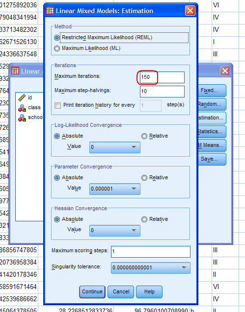
Next, click on the Estimation... button.

Next, change the Maximum iterations from the default (100) to 150 (marked with the red soft rectangle). This step is not technically necessary, but it insures the estimated values match those produced in R using the lme4 package. Then, click the Continue button.

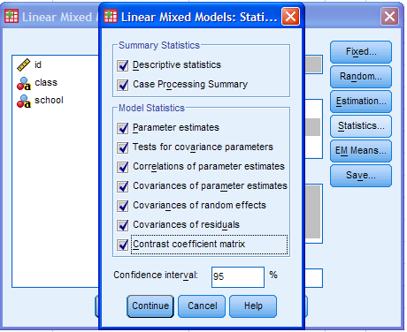
Next, click on the Statistics... button. While some of the options are not necessary (Case Processing Summary), I generally click all of them.

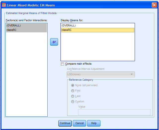
Next, click on the EM Means... button (Estimated Marginal Means). When the (OVERALL) factor is moved to the Display Means for box, the grand mean will be produced. The classRC factor is present (and moved to the Display Means for box) because it is the only factor (categorical variable) included in the model as a fixed effect. The other fixed effects are not categorical and thus do not appear here. Next, click the Continue button.

Next, click on the Save... button. It is generally a good idea to save the Predicted values. The Fixed Predicted Values will be predicted values based solely on the Fixed Effects part of the model; while the lower Predicted Values & Residuals Predicted values will be the whole model's predicted values. Next, click the Continue button.

Then click the Paste button. Your syntax should match what is below. The reason I recommend pasting the syntax is that it takes quite a few clicks to create one of these types of models and it is often the case that multiple models are run during a session and changing variables or options is simply easier in the syntax than pointing and clicking back through all the above steps.

Next, highlight / select all the text in the syntax and then click the green 'run' arrow (marked with the red ellipse).

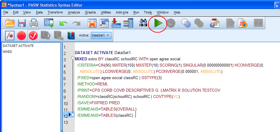
Your output should be the same as what is below.

5. Interpreting the Output.

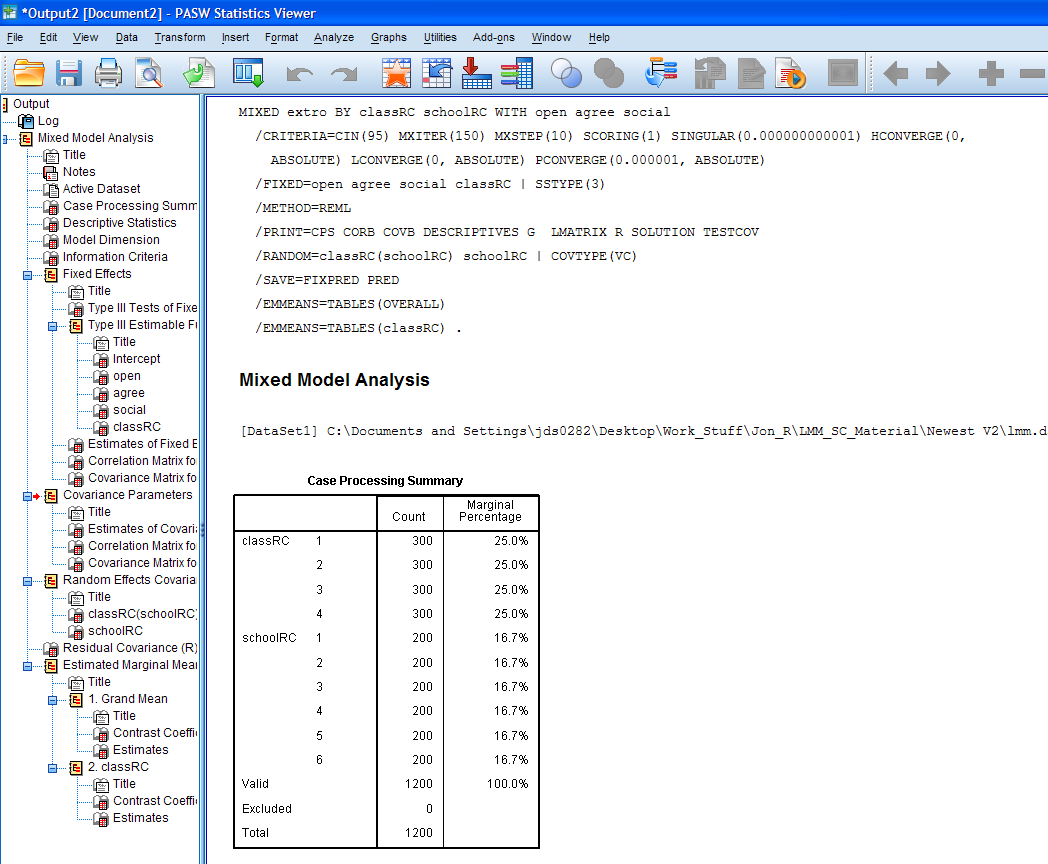
The Case Processing Summary (above) simply shows that the cases are balanced among the categories of the categorical variables and no cases were excluded.

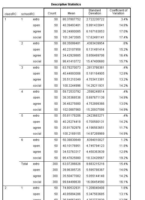
The next, rather large table contains all the descriptive statistics (only the very top of the table is shown here; below).

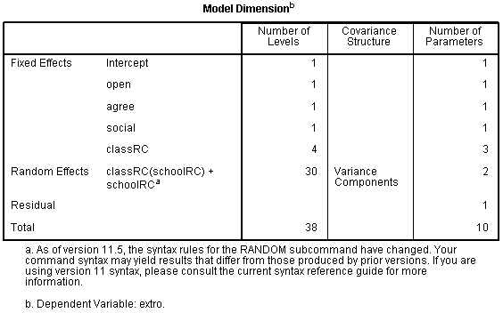
The Model Dimension table (below) simply shows the model in terms of which variables (and their number of levels) are fixed and / or random effects and the number of parameters being estimated.

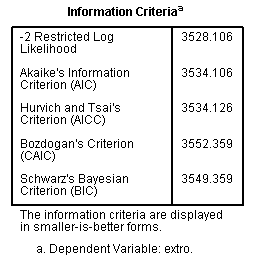
The next table displays fit indices. For each index; the lower the number, the better the model fits the data. Generally I use and recommend the Bayesian Information Criterion (BIC).

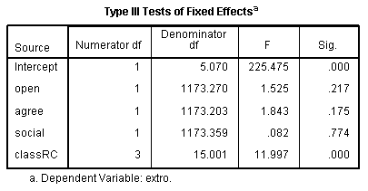
The next table contains the results of the Fixed Effects tests; here we see the intercept and the classRC variables appear to be the main contributors.

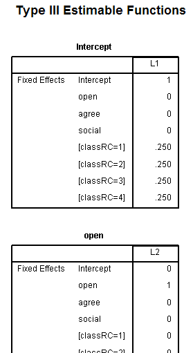
The next 5 tables do not offer much information and simply show each parameter function (only the first and part of the second tables of the five are shown below).

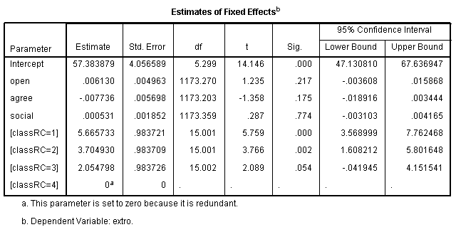
The next table "Estimates of Fixed Effects" (below) is very important and shows the parameter estimates for the Fixed Effects specified in the model. It should be clear, this table and its interpretation are exactly like one would expect from a traditional ordinary least squares linear regression. One thing to note is the way SPSS chooses the reference category for categorical variables. You may have noticed we have been using the classRC and schoolRC variables instead of the original class and school variables in the data set. The RC variables contain the same information as the original variables, they simply have been ReCoded or Reverse Coded so that the output here will match the output produced using the lme4 package in the R programming language. It is important to know that SPSS (and SAS) automatically choose the category with the highest numerical value (or the lowest alphabetical letter) as the reference category for categorical variables. All packages I have used in the R programming language choose the reference category in the more intuitive but opposite way. In the lme4 package (and others I've used) in R, the software automatically picks the lowest numerical value (or the earliest alphabetically letter) as the reference category for categorical variables. This has drastic implications for the intercept estimate and more troubling, the predicted values produced by a model. For example, if this same model is specified with the original variables (not reverse coded) then the Fixed Effects intercept term is 63.049612; so you can imagine how much different the predicted values would be in that model compared to this model where the intercept is 57.383879. Recall from multiple regression, the intercept is interpreted as the mean of the outcome (extro) when all the predictors have a value of zero. The predictor estimates (coefficients or slopes) are interpreted the same way as the coefficients from a traditional regression. For instance, a one unit increase in the predictor Openness to new experiences (open) corresponds to a 0.006130 increase in the outcome Extroversion (extro). Likewise, a one unit increase in the predictor Agreeableness (agree) corresponds to a 0.007736 decrease in the outcome Extroversion (extro). Furthermore, the categorical predictor classRC = 3 has a coefficient of 2.054798; which means, the mean Extroversion score of the third group of classRC (3) is 2.0547978 higher than the mean Extroversion score of the last group of classRC (4). ClassRC (4) was automatically coded as the reference category.

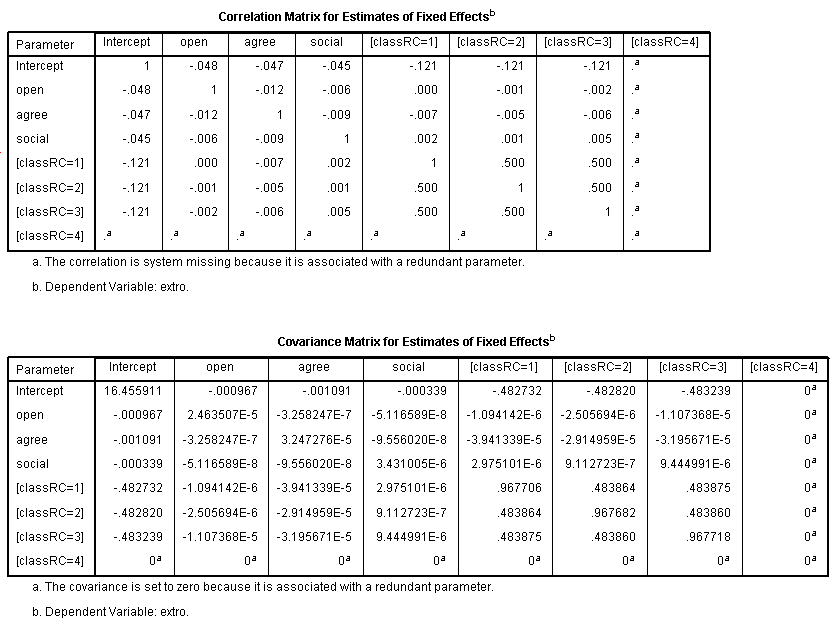
The next 2 tables simply show the correlation matrix and covariance matrix for the fixed effects estimates. We can see that multicollinearity is not an issue among the predictors because, their correlations (and covariances) are quite low (except of course, the categories of the classRC variable which as expected, are related).

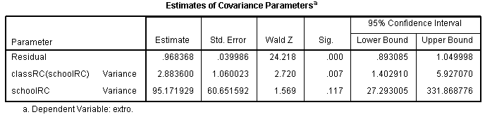
Next, we have the Estimates of Covariance Parameters table (below); which are the parameter estimates for the Random Effects. These are variance estimates (with standard errors, Wald Z test statistics, significance values, and confidence intervals for the variance estimates). Recall the ubiquitous ANOVA summary table where we generally have a total variance estimate (sums of squares) at the bottom, then just above it we have a residual or within groups variance estimate (sums of squares) and then we have each treatment or between groups variance estimate (sums of squares). This table is very much like that, but the total is not displayed and the residual variance estimate is on top. So, we can quickly calculate the total variance estimate: 95.171929 + 2.883600 + .968368 = 99.0239 then we can create an R? type of effect size to gauge the importance of each random effect by dividing the effect's variance estimate by the total variance estimate to arrive at a proportion of variance explained or accounted for by each random effect. This is analogous to an Eta-squared (η?) in standard ANOVA or an R? in regression; it is sometimes referred to (in the linear mixed effects situation) as an Intraclass Correlation Coefficient (ICC, Bartko, 1976; Bliese, 2009). For example, we find that the nested effect of classRC within schoolRC is 2.883600 / 99.0239 = 0.02912024 or simply stated, that random nested effect only accounts for 2.9% of the variance of the random effects. However, the random effect for schoolRC alone accounts for 95.171929 / 99.0239 = 0.9611006 or 96% of the variance of the random effects. If none of the random effects account for a meaningful amount of variance in the random effects (i.e. if the residual variance is larger than the random effect variance estimates), then the random effects should be eliminated from the model and a standard General Linear Model (or Generalized Linear Model) should be fitted (i.e., a model with only the fixed effects). Notice, SPSS does not calculate the standard errors correctly and therefore, the confidence interval estimates and the results of the Wald Z test are NOT valid. The Wald Z test simply divides the estimate by its standard error to arrive at a Z-score to test for significance with the standard normal distribution of Z-scores. However, the standard errors do not match with the standard errors produced when using the lme4 package in the R programming language. The good news is that the variance estimates are correct (do match) and the proportion of variance estimates can be correctly computed and used as effect size measures.

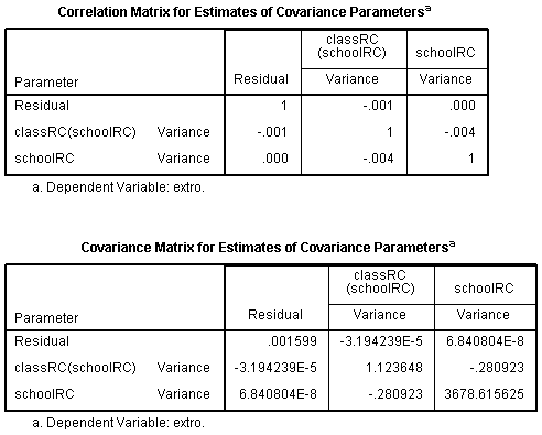
The next two tables simply show the correlation and covariances for the random effect parameter estimates.

The next three tables in the output are the Random Effects Covariance Structure matrices. They are omitted here because they are particularly useless and redundant; because each table simply lists the parameter estimate for each random effect.

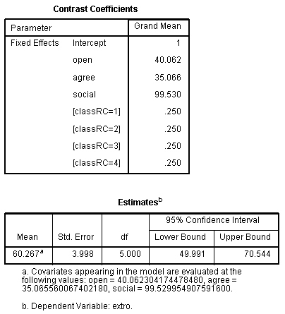
The last part of the output contains tables with the Estimated Marginal means (EM means) for the Grand Mean and ClassRC.

The Grand Mean contrast coefficients table and actual grand mean table (the overall mean of the outcome variable: extro).

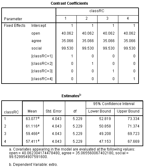
The ClassRC variable's contrast coefficients table and mean extroversion (extro) for each group table.

As with most of the tutorials / pages within this site, this page should not be considered an exhaustive review of the topic covered and it should not be considered a substitute for a good textbook.

References / Resources

Akaike, H. (1974). A new look at the statistical model identification. I.E.E.E. Transactions on Automatic Control, AC 19, 716 – 723. Available at:

Bartko, J. J. (1976). On various intraclass correlation reliability coefficients. Psychological Bulletin, 83, 762-765.

           http://bayes.acs.unt.edu:8083:8083/BayesContent/class/Jon/MiscDocs/Bartko_1976.pdf

Bates, D., & Maechler, M. (2010). Package ‘lme4’. Reference manual for the package, available at:

           http://cran.r-project.org/web/packages/lme4/lme4.pdf

Bates, D. (2010). Linear mixed model implementation in lme4. Package lme4 vignette, available at:

            http://cran.r-project.org/web/packages/lme4/vignettes/Implementation.pdf

Bates, D. (2010). Computational methods for mixed models. Package lme4 vignette, available at:

http://cran.r-project.org/web/packages/lme4/vignettes/Theory.pdf

Bates, D. (2010). Penalized least squares versus generalized least squares representations of linear mixed models. Package lme4 vignette, available at:

http://cran.r-project.org/web/packages/lme4/vignettes/PLSvGLS.pdf

Bliese, P. (2009). Multilevel modeling in R: A brief introduction to R, the multilevel package and the nlme package. Available at:

           http://cran.r-project.org/doc/contrib/Bliese_Multilevel.pdf

Draper, D. (1995). Inference and hierarchical modeling in the social sciences. Journal of Educational and Behavioral Statistics, 20(2), 115 - 147. Available at:

Fox, J. (2002). Linear mixed models: An appendix to “An R and S-PLUS companion to applied regression”. Available at:

http://cran.r-project.org/doc/contrib/Fox-Companion/appendix-mixed-models.pdf

Gelman, A. (2005). Analysis of variance -- why it is more important than ever. The Annals of Statistics, 33(1), 1 -- 53. Available at:

            http://bayes.acs.unt.edu:8083:8083/BayesContent/class/Jon/MiscDocs/Gelman_2005.pdf

Hofmann, D. A., Griffin, M. A., & Gavin, M. B. (2000). The application of hierarchical linear modeling to organizational research. In K. J. Klein (Ed.), Multilevel theory, research, and methods in organizations: Foundations, extensions, and new directions (p. 467 - 511). San Francisco, CA: Jossey-Bass. Available at:

Raudenbush, S. W. (1995). Reexamining, reaffirming, and improving application of hierarchical models. Journal of Educational and Behavioral Statistics, 20(2), 210 - 220. Available at:

Raudenbush, S. W. (1993). Hierarchical linear models and experimental design. In L. Edwards (Ed.), Applied analysis of variance in behavioral science (p. 459 - 496). New York: Marcel Dekker. Available at:

Rogosa, D., & Saner, H. (1995). Longitudinal data analysis examples with random coefficient models. Journal of Educational and Behavioral Statistics, 20(2), 149 - 170. Available at:

Schwarz, G. (1978). Estimating the dimension of a model. Annals of Statistics, 6, 461 – 464. Available at:

Return to the SPSS Short Course