|
Logistic Regression (Binary)
Binary (also called binomial) Logistic regression
is appropriate when the outcome is a dichotomous variable (i.e.
categorical with only two categories) and the predictors are of any
type: nominal, ordinal, and / or interval/ratio (numeric). Either
Multi-nomial Logistic Regression or Discriminant Function Analysis is
appropriate when the outcome variable is polytomous (i.e. categorical
with more than two categories). Standard multiple regression can only
accommodate an outcome variable which is continuous or nearly
continuous (i.e. interval/ratio in scale) and it works best with
continuous or nearly continuous predictor variables. Although standard
regression can accommodate categorical predictors using one of the
following strategies for those types of predictors: dummy coding,
effects coding, orthogonal coding, or criterion coding. Binary logistic
and multinomial logistic regression can also accommodate categorical
predictors, but categorical predictors must be identified in the menu
system when the analysis is being specified.
For the duration of this tutorial we will be using
the
logreg1.sav
file; which contains 1 dichotomous categorical outcome variable (y) and
4 predictor variables (x1 - x4). The outcome (y) contains the values 0
and 1.
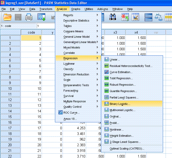
Begin by clicking on Analyze, Regression, Binary
Logistic...
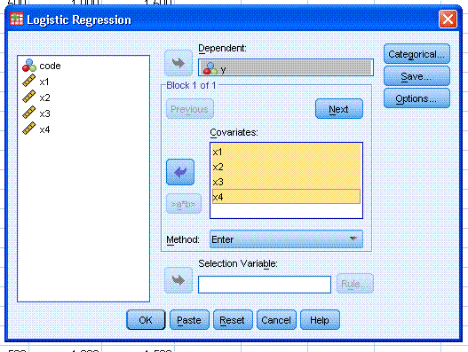
Next, highlight / select the outcome variable (y)
and use the top arrow button to move it to the Dependent: box. Then,
highlight the four predictor variables (x1, x2, x3, x4) and use the
second arrow button to move them to the Covariates: box. Notice, if one
or more of the predictors was categorical, we would need to click on
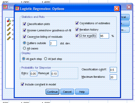
the Categorical... button to specify them as such. Click on the
Options... button and select Classification plots, Hosmer-Lemeshow
goodness-of-fit, Casewise listing of residuals, Correlations of
estimates, Iteration history, and CI for exp(B):. Then, click the
Continue button, then click the OK button.
The output should be similar to what is displayed
below.
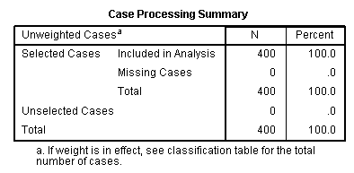
The Case Processing Summary table provides an
overview of missing data; here there was no missing data. The Dependent
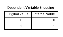
Variable Encoding table shows how the outcome variable was coded, if it
was coded. Here, the outcome variable was not coded; therefore, the
values are listed in both columns. If, for example, the outcome
variable represented responses yes and no, then the left column
(Original Value) would show the associated value labels, 'yes' and 'no'
while the right column (Internal Value) would show the values 0 and 1
for each. By default, the binary logistic regression predicts the odds
of membership in the outcome category with the highest value; here
predicting membership in the 1 value, as opposed to membership in the 0
value.
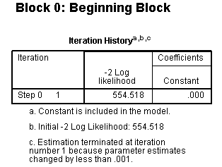
The Beginning Block evaluates our model with only
the constant in the equation (sometimes called the null model). The
constant is analogous to the y-intercept in OLS regression. The
iteration history was specified in the options, is displayed throughout
the output file. The first Iteration History table (directly below)
shows that estimation was terminated at iteration # 1 because the
parameter estimates did not change by more than 0.001. The -2 Log
likelihood (-2 LL) is a likelihood ratio and represents the unexplained
variance in the outcome variable. Therefore, the smaller the value, the
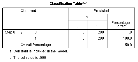
better the fit. The Classification Table shows how well our null model
correctly classifies cases. The rows represent the number of cases in
each category in the actual data and the columns represent the number
of cases in each category as classified by the null model. The key
piece of information is the overall percentage in the lower right
corner which shows our null model is only 50% accurate; which is equal
to the accuracy of random guessing.
The Variables in the Equation table shows the
logistic coefficient (B) associated with the intercept as it is
included in the model. This table is similar to and contains analogous
information as the coefficients table in a standard regression. The
logistic coefficient for the constant is similar to the y-intercept
term in standard regression. The Wald statistic is a chi-square 'type'
of statistic and is used to test the significance of the variable in
the model. The Exp(B) refers to the change in odds ratio attributed to
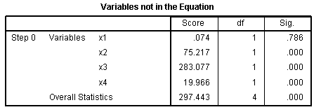
the variable. The Variables not in the Equation table simply lists the
Wald test score, df, and p-value
for each of the variables not included in the
beginning block model. Notice the Overall Statistics is not a total,
but rather an estimate of overall Wald statistic associated with the
model had all the variables been included.

The number of blocks will increase with and
correspond to the number of
blocks of covariates or predictors entered into the model.
Meaning, when specifying the variable for inclusion into the model, you
notice above in the second figure (Logistic Regression dialog box) we
could have clicked the Next button and entered more variables as a
distinct block (as is done in sequential or hierarchical
regression). Here, we only have one set of predictors so
there is only the intercept model block (Block 0) above and the
complete model (Block 1) below.
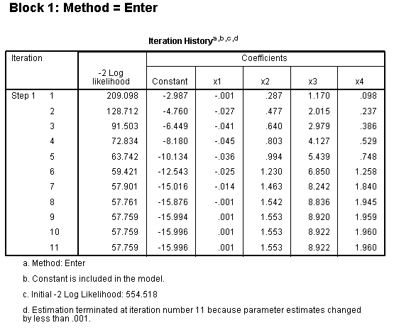
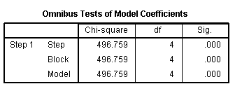
The iteration history (above) was specified in the
options, is displayed throughout the output file. The Iteration History
table (above left) shows that estimation was terminated at iteration #
11 because the parameter estimates did not change by more than 0.001.
The -2 LL is a likelihood ratio and represents the unexplained variance
in the outcome variable. Therefore, the smaller the value, the better
the fit. Notice here the -2 LL (57.759) is substantially lower than
that given above for the null model (554.518). The Omnibus Tests of
Model Coefficients table reports the chi-square associated with each
step in a stepwise model. Here, there is only one step from the
constant model to the block containing predictors so all three values
are the same. The significance value or p-value
indicates our model (Block 1; with predictors) is significantly
different from the constant only model; meaning there is a significant
effect for the combined predictors on the outcome variable.
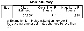

The Model Summary table displays the -2 LL as was
shown and discussed directly above. The two R? estimates
are not truly R?
estimates; they are pseudo-R?; meaning they are
analogous to R?
in standard multiple regression, but do not carry the same
interpretation. They are not representative of the amount of variance
in the outcome variable accounted for by all the predictor variables.
The Nagelkerke estimate is calculated in such a way as to be
constrained between 0 and 1. So, it can be evaluated as indicating
model fit; with a better model displaying a value closer to 1. The
larger Cox & Snell estimate is the better the model; but it can
be greater than 1. These metrics should be interpreted with caution and
although not ignored, they offer little confidence in interpreting the
model fit. The Hosmer and Lemeshow Test table (above right) is the
preferred test of goodness-of-fit. As with most chi-square based tests
however, it is prone to inflation as sample size increases. Here, we
see model fit is acceptable
χ?
(9) = 14.559, p = .068, which indicates our model
predicts values not significantly different from what we observed. To
be clear, you want the p-value to be greater
than your established cutoff (generally 0.05) to indicate
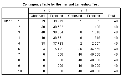
good fit. The Contingency Table for Hosmer and Lemeshow Test (below
left) simply shows the observed and expected values for each category
of the outcome variable as used to calculate the Hosmer and Lemeshow
chi-square.
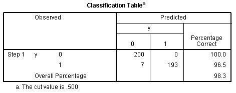
The Classification Table (above right) shows how
well our full model correctly classifies cases. A perfect model would
show only values in the diagonal--correctly classifying all cases.
Adding across the rows represents the number of cases in each category
in the actual data and adding down the columns represents the number of
cases in each category as classified by the full model. The key piece
of information is the overall percentage in the lower right corner
which shows our model (with all predictors & the constant) is
98.3% accurate; which is excellent. One way of assessing the model's
fit is to compare the overall percentage in the full model's table to
the overall percentage in the null model table. Another, more highly
regarded way is to compare the full model's overall percentage to the
chance percentage (50% in this example) plus 25% = 75%. Note,
chance percentage can be weighted by the proportion of cases in each
category of the outcome variable; thus making it more conservative. For
instance, if we had 250 cases (62.5%) in the 1 category and 150 cases
(37.5%) in the 0 category, then we would square and sum those
proportions to arrive at a more conservative chance percentage for
comparison (53.2%). Taking the weighted chance percentage and adding
25% brings the comparison to 78.2 %; still far below what our full
model is capable of.
Weighted chance percentage: .625? + .375? = .391 + .141 = .532 =
53.2%

The Variables in the Equation table (above), shows
the logistic coefficient (B) for each predictor variable. The logistic
coefficient is the expected amount of change in the logit for each one
unit change in the predictor. The logit is what is being predicted; it
is the odds of membership in the category of the outcome variable with
the numerically higher value (here a 1, rather than 0). The closer a
logistic coefficient is to zero, the less influence it has in
predicting the logit. The table also displays the standard error, Wald
statistic, df, Sig. (p-value);
as well as the Exp(B) and confidence interval for the Exp(B). The Wald
test (and associated p-value) is used to evaluate
whether or not the logistic coefficient is different than zero. The
Exp(B) is the odds ratio associated with each predictor. We expect
predictors which increase the logit to display Exp(B) greater than 1.0,
those predictors which do not have an effect on the logit will display
an Exp(B) of 1.0 and predictors which decease the logit will have
Exp(B) values less than 1.0. Note that the Exp(B) is wildly large for
the x3 predictor. This is due to a combination of the strong
relationship between that variable and the outcome variable; and the
fact that x3 is nearly categorical itself. Generally, when using
continuous variables as predictors, you will not see such large
Exp(B).
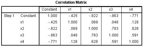
The Correlation Matrix table simply shows the
correlations between each of the predictor variables and the constant
(note the outcome is not included).
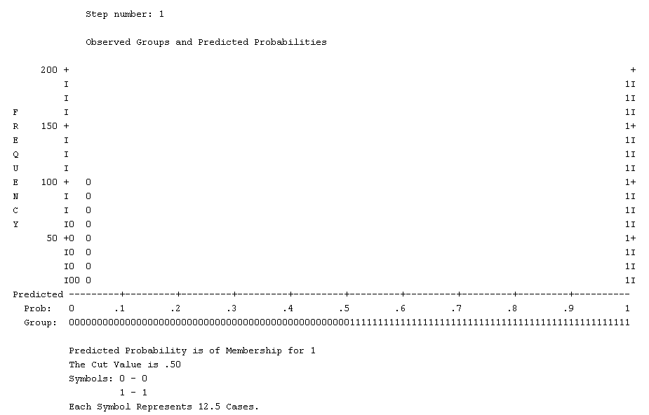
The graph (above) shows how our full model
predicts membership. It is unusually clear in the middle because our
model was so accurate. When a model is less accurate, more symbols
(here 1 and 0) would appear in the middle, displaying their probability
(x-axis). The better the model, the clearer the middle of the graph.
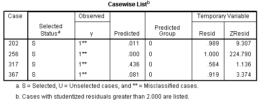
The Casewise List table displays cases which were
incorrectly classified by the model. Here, we only have four cases
mis-classified.
As with most of the tutorials / pages within this
site, this page should not be considered an exhaustive review of the
topic covered and it should not be considered a substitute for a good
textbook.
|


