MODULE 9

Multinomial Logistic regression is appropriate when the outcome is a polytomous variable (i.e. categorical with more than two categories) and the predictors are of any type: nominal, ordinal, and / or interval/ratio (numeric). Discriminant Function Analysis (DFA) may be used in the same situation; but DFA requires adherence to more assumptions and therefore, multinomial logistic regression is often preferred when the outcome variable is categorical. Multinomial logistic regression does not require the use of a coding strategy (i.e. dummy coding, effects coding, etc.) for including categorical predictors in the model. Categorical predictor variables can be included directly as factors in the multinomial logistic regression dialog menu box. 

For the duration of this tutorial we will be using the MultiNomReg.sav file; which contains 1 polytomous categorical outcome variable (y) and 3 continuous predictor variables (x1 - x3); and 600 cases. 

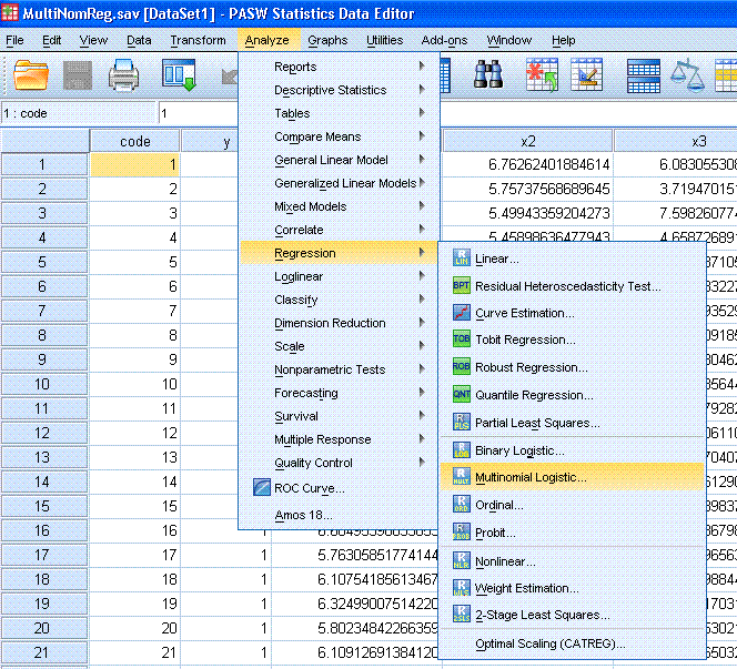
Begin by clicking on Analyze, Regression, Multinomial Logistic...

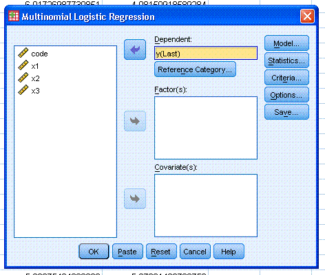
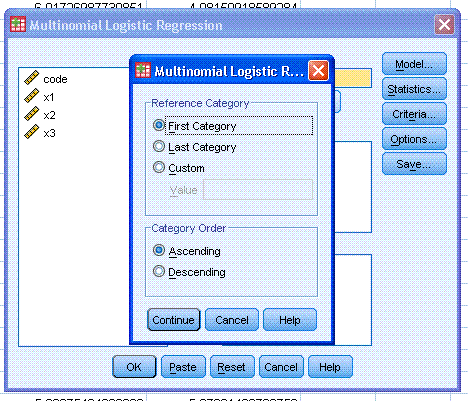
Next, highlight / select the outcome variable (y) and use the top arrow button to move it to the Dependent: box. Next, click on the Reference Category... button and select First Category. Then click the Continue button.

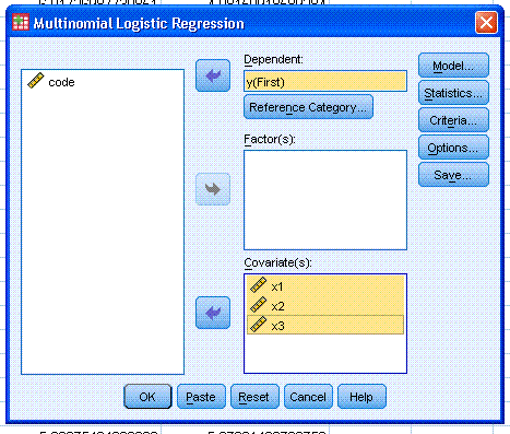
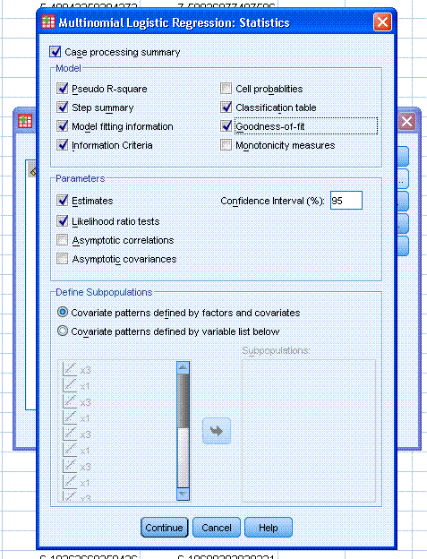
Next, select all three of the predictor variables (x1, x2, x3) and use the bottom arrow button to move them to the Covariate(s): box. Notice here, if we had any categorical predictors, we would move them to the Factor(s): box. Next, click the Statistics... button and select the following. The cell probabilities will not be displayed if selected because, with only continuous predictors in the model, too many cells would be produced. Also, the Monotonicity measures table will not be needed because our outcome variable has more than two categories. Next, click the Continue button, then click the OK button to complete the analysis.

The output should be similar to what is displayed below.

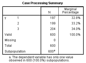
The Case Processing Summary table simply shows how many cases or observations were in each category of the outcome variable (as well as their percentages). It also shows if there was any missing data. The Model Fitting Information table (above right) shows various indices for assessing the intercept only model (sometimes referred to as the null model) and the final model which includes all the predictors and the intercept (sometimes called the full model). Both the Akaike Information Criterion (AIC) and the Bayesian Information Criterion (BIC) are information theory based model fit statistics. Lower values of indicate better model fit and both can be below zero (i.e. larger negative values indicate better fit than values closer to zero). The BIC tends to be more conservative. Similarly, the -2 Log Likelihood (-2LL) should be lower for the the full model than it is for the null model; lower values indicate better fit. The -2 LL is a likelihood ratio and represents the unexplained variance in the outcome variable. Therefore, the smaller the value, the better the fit. The Likelihood Ratio chi-square test is alternative test of goodness-of-fit. As with most chi-square based tests however, it is prone to inflation as sample size increases. Here, we see model fit is significant χ² (6) = 1291.00, p < .001, which indicates our full model predicts significantly better, or more accurately, than the null model. To be clear, you want the p-value to be less than your established cutoff (generally 0.05) to indicate good fit.

The Goodness-of-Fit table provides further evidence of good fit for our model. Again, both the Pearson and Deviance statistics are chi-square based methods and subject to inflation with large samples. Here, we interpret lack of significance as indicating good fit. To be clear, you want the p-value to be greater than your established cutoff (generally 0.05) to indicate good fit. The Pseudo R-Square table displays three metrics which have been developed to provide a number familiar to those who have used traditional, standard multiple regression. They are treated as measures of effect size, similar to how R² is treated in standard multiple regression. However, these metrics do not represent the amount of variance in the outcome variable accounted for by the predictor variables. Higher values indicate better fit, but they should be interpreted with caution.

The statistics in the Likelihood Ratio Tests table are the same types as those reported for the null and full models above in the Model Fitting Information table. Here however, each element of the model is being compared to the full model in such a way as to allow the research to determine if it (each element) should be included in the full model. In other words, does each element (predictor) contributed meaningfully to the full effect. For instance, we see that the x3 predictor displays a non-significant (p = .110) chi-square which indicates x3 could be dropped from the model and the overall fit would NOT be significantly reduced. To be clear, if the p-value is less than your established cutoff (generally 0.05) for a predictor then that predictor contributes significantly to the full (final) model.    

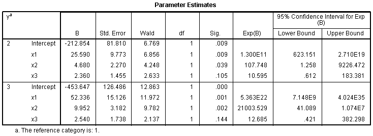
The Parameter Estimates table (above), shows the logistic coefficient (B) for each predictor variable for each alternative category of the outcome variable. Alternative category meaning, not the reference category. The logistic coefficient is the expected amount of change in the logit for each one unit change in the predictor. The logit is what is being predicted; it is the odds of membership in the category of the outcome variable which has been specified (here the first value: 1 was specified, rather than the alternative values 2 or 3). The closer a logistic coefficient is to zero, the less influence the predictor has in predicting the logit. The table also displays the standard error, Wald statistic, df, Sig. (p-value); as well as the Exp(B) and confidence interval for the Exp(B). The Wald test (and associated p-value) is used to evaluate whether or not the logistic coefficient is different than zero. The Exp(B) is the odds ratio associated with each predictor. We expect predictors which increase the logit to display Exp(B) greater than 1.0, those predictors which do not have an effect on the logit will display an Exp(B) of 1.0 and predictors which decease the logit will have Exp(B) values less than 1.0. As an example, we can see that a one unit change in x3 does not significantly change the odds of being classified in the first category of the outcome variable relative to the second or third categories of the outcome variable, while controlling for the influence of the other predictors.

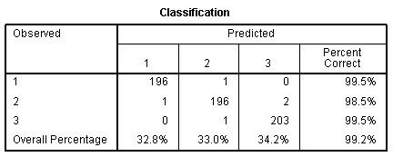
The Classification Table (above) shows how well our full model correctly classifies cases. A perfect model would show only values on the diagonal--correctly classifying all cases. Adding across the rows represents the number of cases in each category in the actual data and adding down the columns represents the number of cases in each category as classified by the full model. The key piece of information is the overall percentage in the lower right corner which shows our model (with all predictors & the constant) is 99.2% accurate; which is excellent.

As with most of the tutorials / pages within this site, this page should not be considered an exhaustive review of the topic covered and it should not be considered a substitute for a good textbook.

Return to the SPSS Short Course